# load libraries used in analysis
library(tidyverse)
library(patchwork)
library(jtools)
library(kableExtra)Statistical Analysis
# read in data generated from geospatial analysis
blackout_census_data <- read_csv("data/census_tract_blackout_data_df.csv")
Linear Regression
Linear regression was used to model the relationship between percent of houses that lost power and selected data from the U.S. Census Bureau’s American Community Survey (ACS). All data are aggregated to the census tract level.
Race
Percent white
# linear regression model
model_pct_white <- lm(data = blackout_census_data, pct_houses_that_lost_power ~ pct_white)

#plot
plot_model_pct_white <- ggplot(data = blackout_census_data, aes(x = pct_white, y = pct_houses_that_lost_power)) +
  geom_point(size = 0.5) +
  geom_smooth(method = lm, formula = y~x, se = FALSE) +
  theme_classic() +
  labs(x = "% white", y = "% of houses that lost power")
plot_model_pct_white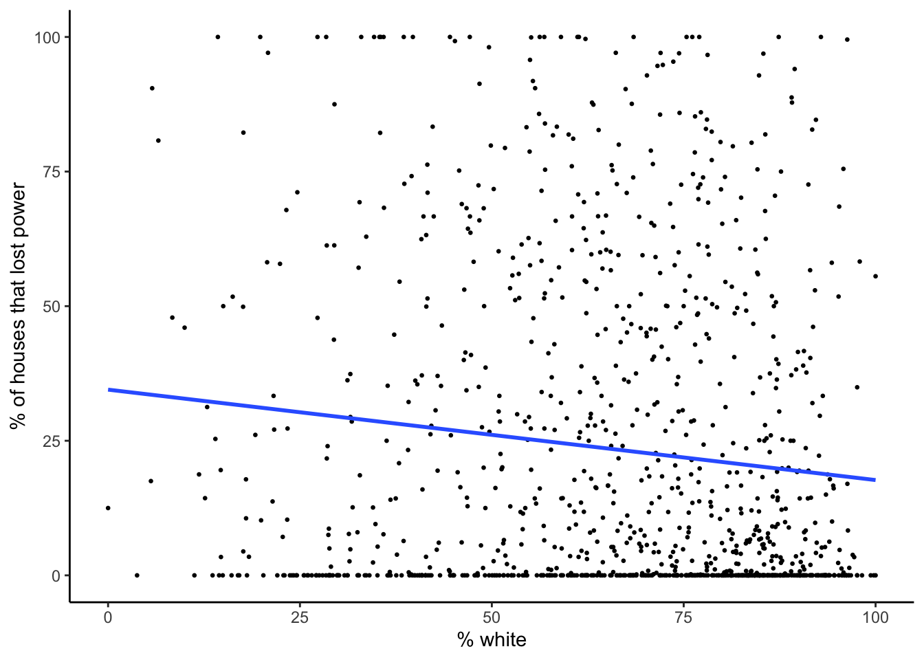
Code for model summary result values
# model summary
summary_model_pct_white <- summary(model_pct_white)

# extract model coefficients
slope_coef_white <- round(summary_model_pct_white$coefficients["pct_white", "Estimate"], digits = 3)

std_err_white <- round(summary_model_pct_white$coefficients["pct_white", "Std. Error"], digits = 3)

p_value_white <- format(summary_model_pct_white$coefficients["pct_white", "Pr(>|t|)"], scientific = FALSE, digits = 2)

# confidence intervals
ci_95_lower_white <- round(confint(model_pct_white, level = 0.95)[2, 1], digits = 3)
ci_95_upper_white <- round(confint(model_pct_white, level = 0.95)[2, 2], digits = 3)

# r-squared value
r_sqrd_white <- round(summary_model_pct_white$r.squared, digits = 3)
Percent black
# linear regression model
model_pct_black <- lm(data = blackout_census_data, pct_houses_that_lost_power ~ pct_black)

# plot
plot_model_pct_black <- ggplot(data = blackout_census_data, aes(x = pct_black, y = pct_houses_that_lost_power)) +
  geom_point(size = 0.5) +
  geom_smooth(method = lm, formula = y~x, se = FALSE) +
  theme_classic() +
  labs(x = "% black", y = "% of houses that lost power")
plot_model_pct_black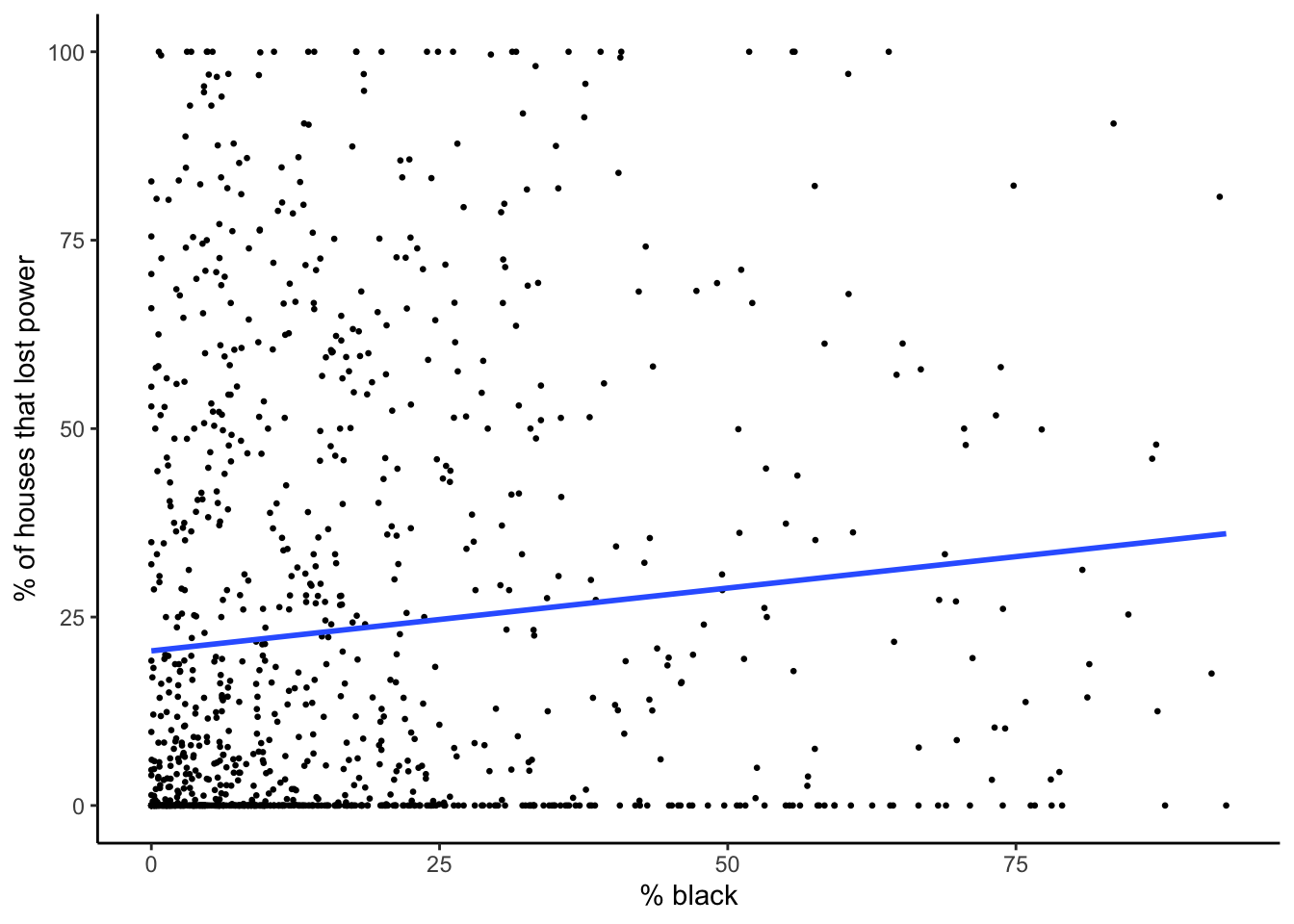
Code for model summary result values
# model summary
summary_model_pct_black <- summary(model_pct_black)

# extract model coefficients
slope_coef_black <- round(summary_model_pct_black$coefficients["pct_black", "Estimate"], digits = 3)

std_err_black <- round(summary_model_pct_black$coefficients["pct_black", "Std. Error"], digits = 3)

p_value_black <- format(summary_model_pct_black$coefficients["pct_black", "Pr(>|t|)"], scientific = FALSE, digits = 2)

# confidence intervals
ci_95_lower_black <- round(confint(model_pct_black, level = 0.95)[2, 1], digits = 3)
ci_95_upper_black <- round(confint(model_pct_black, level = 0.95)[2, 2], digits = 3)

# r-squared value
r_sqrd_black <- round(summary_model_pct_black$r.squared, digits = 3)
Percent native american
# linear regression model
model_pct_am_native <- lm(data = blackout_census_data, pct_houses_that_lost_power ~ pct_am_native)

# plot
plot_model_pct_am_native <- ggplot(data = blackout_census_data, aes(x = pct_am_native, y = pct_houses_that_lost_power)) +
  geom_point(size = 0.5) +
  geom_smooth(method = lm, formula = y~x, se = FALSE) +
  theme_classic() +
  labs(x = "% native american", y = "% of houses that lost power")
plot_model_pct_am_native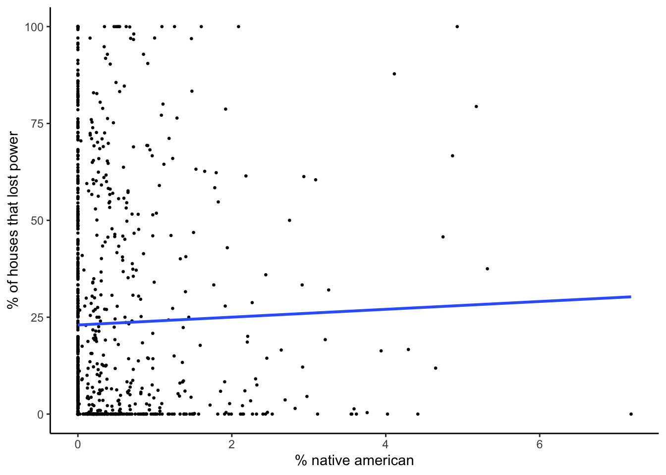
Code for model summary result values
# model summary
summary_model_pct_am_native <- summary(model_pct_am_native)

# extract model coefficients
slope_coef_am_native <- round(summary_model_pct_am_native$coefficients["pct_am_native", "Estimate"], digits = 3)

std_err_am_native <- round(summary_model_pct_am_native$coefficients["pct_am_native", "Std. Error"], digits = 3)

p_value_am_native <- format(summary_model_pct_am_native$coefficients["pct_am_native", "Pr(>|t|)"], scientific = FALSE, digits = 2)

# confidence intervals
ci_95_lower_am_native <- round(confint(model_pct_am_native, level = 0.95)[2, 1], digits = 3)
ci_95_upper_am_native <- round(confint(model_pct_am_native, level = 0.95)[2, 2], digits = 3)

# r-squared value
r_sqrd_am_native <- round(summary_model_pct_am_native$r.squared, digits = 3)
Percent asian
# linear regression model
model_pct_asian <- lm(data = blackout_census_data, pct_houses_that_lost_power ~ pct_asian)

# plot
plot_model_pct_asian <- ggplot(data = blackout_census_data, aes(x = pct_asian, y = pct_houses_that_lost_power)) +
  geom_point(size = 0.5) +
  geom_smooth(method = lm, formula = y~x, se = FALSE) +
  theme_classic() +
  labs(x = "% asian", y = "% of houses that lost power")
plot_model_pct_asian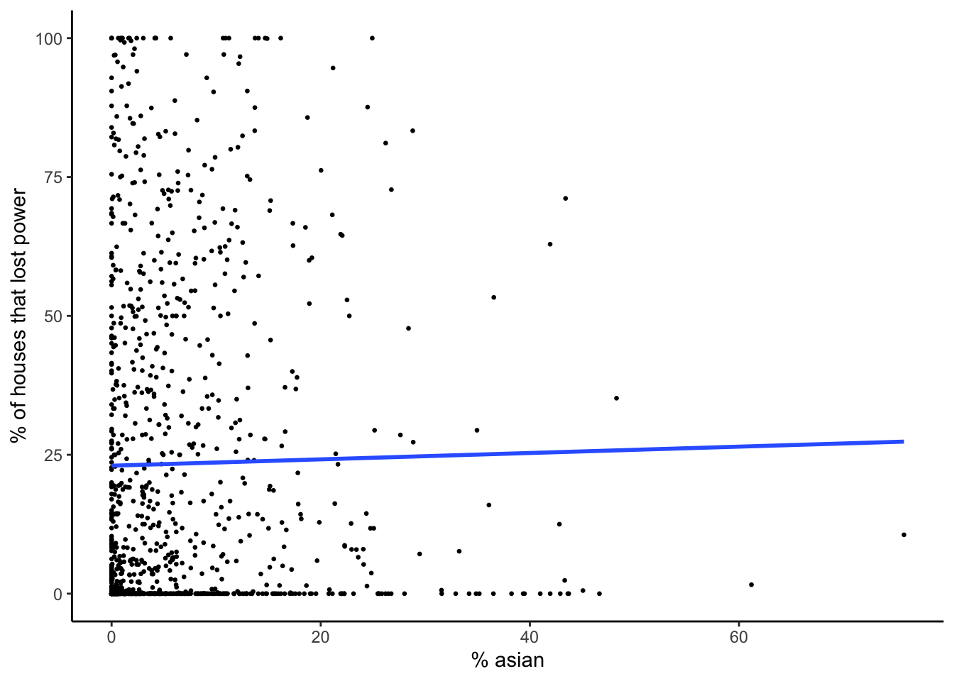
Code for model summary result values
# model summary
summary_model_pct_asian <- summary(model_pct_asian)

# extract model coefficients
slope_coef_asian <- round(summary_model_pct_asian$coefficients["pct_asian", "Estimate"], digits = 3)

std_err_asian <- round(summary_model_pct_asian$coefficients["pct_asian", "Std. Error"], digits = 3)

p_value_asian <- format(summary_model_pct_asian$coefficients["pct_asian", "Pr(>|t|)"], scientific = FALSE, digits = 2)

# confidence intervals
ci_95_lower_asian <- round(confint(model_pct_asian, level = 0.95)[2, 1], digits = 3)
ci_95_upper_asian <- round(confint(model_pct_asian, level = 0.95)[2, 2], digits = 3)

# r-squared value
r_sqrd_asian <- round(summary_model_pct_asian$r.squared, digits = 3)
Percent hispanic / latino
# linear regression model
model_pct_hispanic_latino <- lm(data = blackout_census_data, pct_houses_that_lost_power ~ pct_hispanic_latino)

# plot
plot_model_pct_hispanic_latino <- ggplot(data = blackout_census_data, aes(x = pct_hispanic_latino, y = pct_houses_that_lost_power)) +
  geom_point(size = 0.5) +
  geom_smooth(method = lm, formula = y~x, se = FALSE) +
  theme_classic() +
  labs(x = "% hispanic / latino", y = "% of houses that lost power")
plot_model_pct_hispanic_latino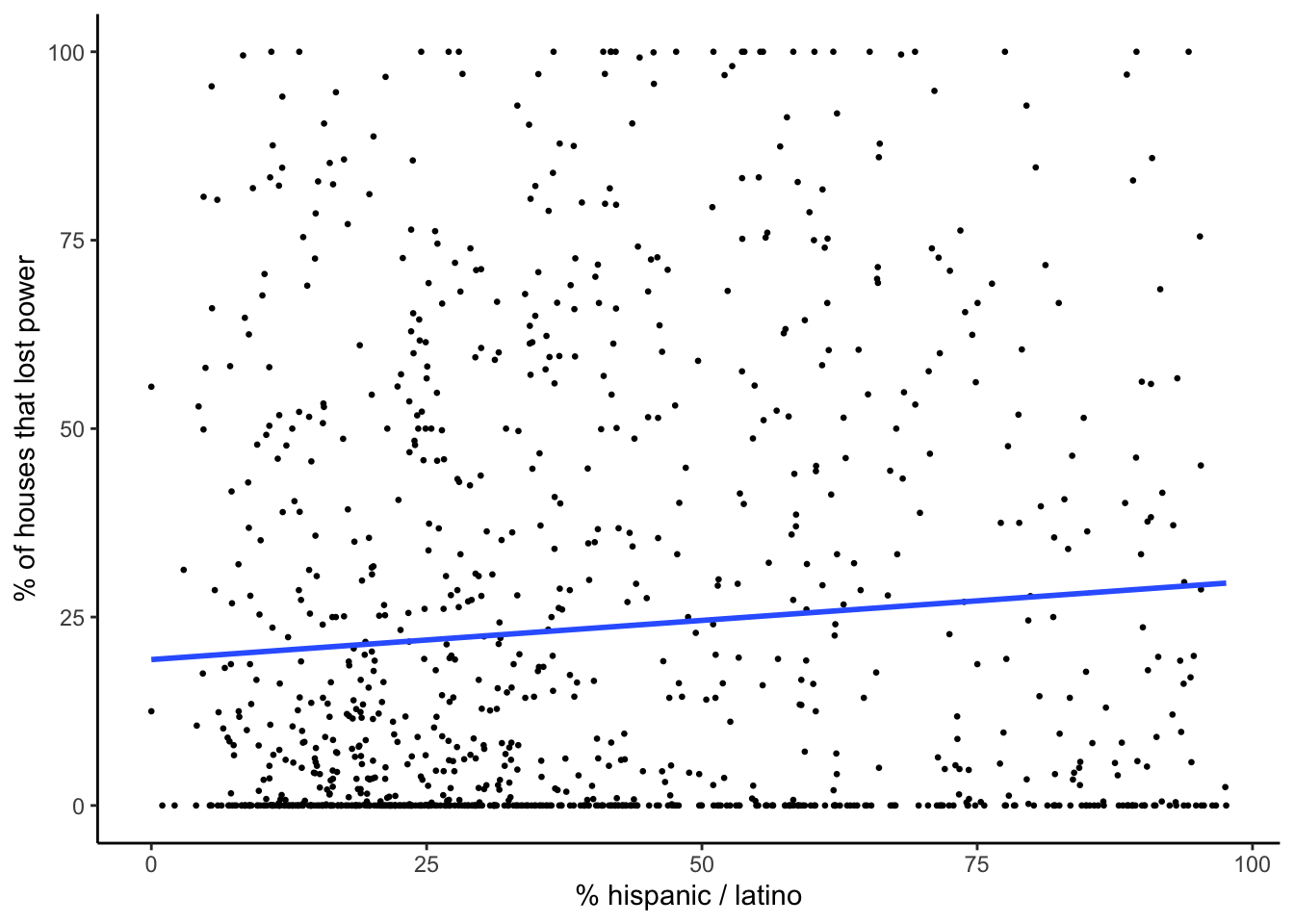
Code for model summary result values
# model summary
summary_model_pct_hispanic_latino <- summary(model_pct_hispanic_latino)

# extract model coefficients
slope_coef_hispanic_latino <- round(summary_model_pct_hispanic_latino$coefficients["pct_hispanic_latino", "Estimate"], digits = 3)

std_err_hispanic_latino <- round(summary_model_pct_hispanic_latino$coefficients["pct_hispanic_latino", "Std. Error"], digits = 3)

p_value_hispanic_latino <- format(summary_model_pct_hispanic_latino$coefficients["pct_hispanic_latino", "Pr(>|t|)"], scientific = FALSE, digits = 2)

# confidence intervals
ci_95_lower_hispanic_latino <- round(confint(model_pct_hispanic_latino, level = 0.95)[2, 1], digits = 3)
ci_95_upper_hispanic_latino <- round(confint(model_pct_hispanic_latino, level = 0.95)[2, 2], digits = 3)

# r-squared value
r_sqrd_hispanic_latino <- round(summary_model_pct_hispanic_latino$r.squared, digits = 3)
Race summary plots
model_plots_race <- (plot_model_pct_white | plot_model_pct_black | plot_model_pct_am_native) /
  (plot_model_pct_asian | plot_model_pct_hispanic_latino | plot_spacer()) +
  plot_annotation(title = "Lineral Regression Models of Power Outages vs. Race")

model_plots_race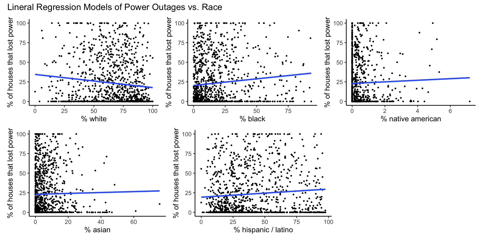
Age
Percent 65 and older
# linear regression model
model_pct_65_and_over <- lm(data = blackout_census_data, pct_houses_that_lost_power ~ pct_65_and_over)

# plot
plot_model_pct_65_and_over <- ggplot(data = blackout_census_data, aes(x = pct_65_and_over, y = pct_houses_that_lost_power)) +
  geom_point(size = 0.5) +
  geom_smooth(method = lm, formula = y~x, se = FALSE) +
  theme_classic() +
  labs(x = "% 65 and older", y = "% of houses that lost power")
plot_model_pct_65_and_over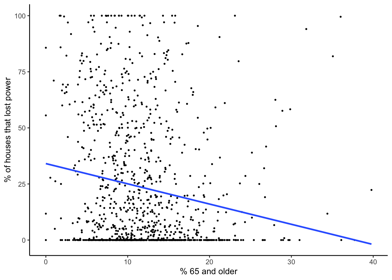
Code for model summary result values
# model summary
summary_model_pct_65_and_over <- summary(model_pct_65_and_over)

# extract model coefficients
slope_coef_pct_65_and_over <- round(summary_model_pct_65_and_over$coefficients["pct_65_and_over", "Estimate"], digits = 3)

std_err_pct_65_and_over <- round(summary_model_pct_65_and_over$coefficients["pct_65_and_over", "Std. Error"], digits = 3)

p_value_pct_65_and_over <- format(summary_model_pct_65_and_over$coefficients["pct_65_and_over", "Pr(>|t|)"], scientific = FALSE, digits = 2)

# confidence intervals
ci_95_lower_pct_65_and_over <- round(confint(model_pct_65_and_over, level = 0.95)[2, 1], digits = 3)
ci_95_upper_pct_65_and_over <- round(confint(model_pct_65_and_over, level = 0.95)[2, 2], digits = 3)

# r-squared value
r_sqrd_65_and_over <- round(summary_model_pct_65_and_over$r.squared, digits = 3)
Percent children under 18
# linear regression model
model_pct_children_under_18 <- lm(data = blackout_census_data, pct_houses_that_lost_power ~ pct_children_under_18)

# plot
plot_model_pct_children_under_18 <- ggplot(data = blackout_census_data, aes(x = pct_children_under_18, y = pct_houses_that_lost_power)) +
  geom_point() +
  geom_smooth(method = lm, formula = y~x, se = FALSE) +
  theme_classic() +
  labs(x = "% children under 18", y = "% of houses that lost power")
plot_model_pct_children_under_18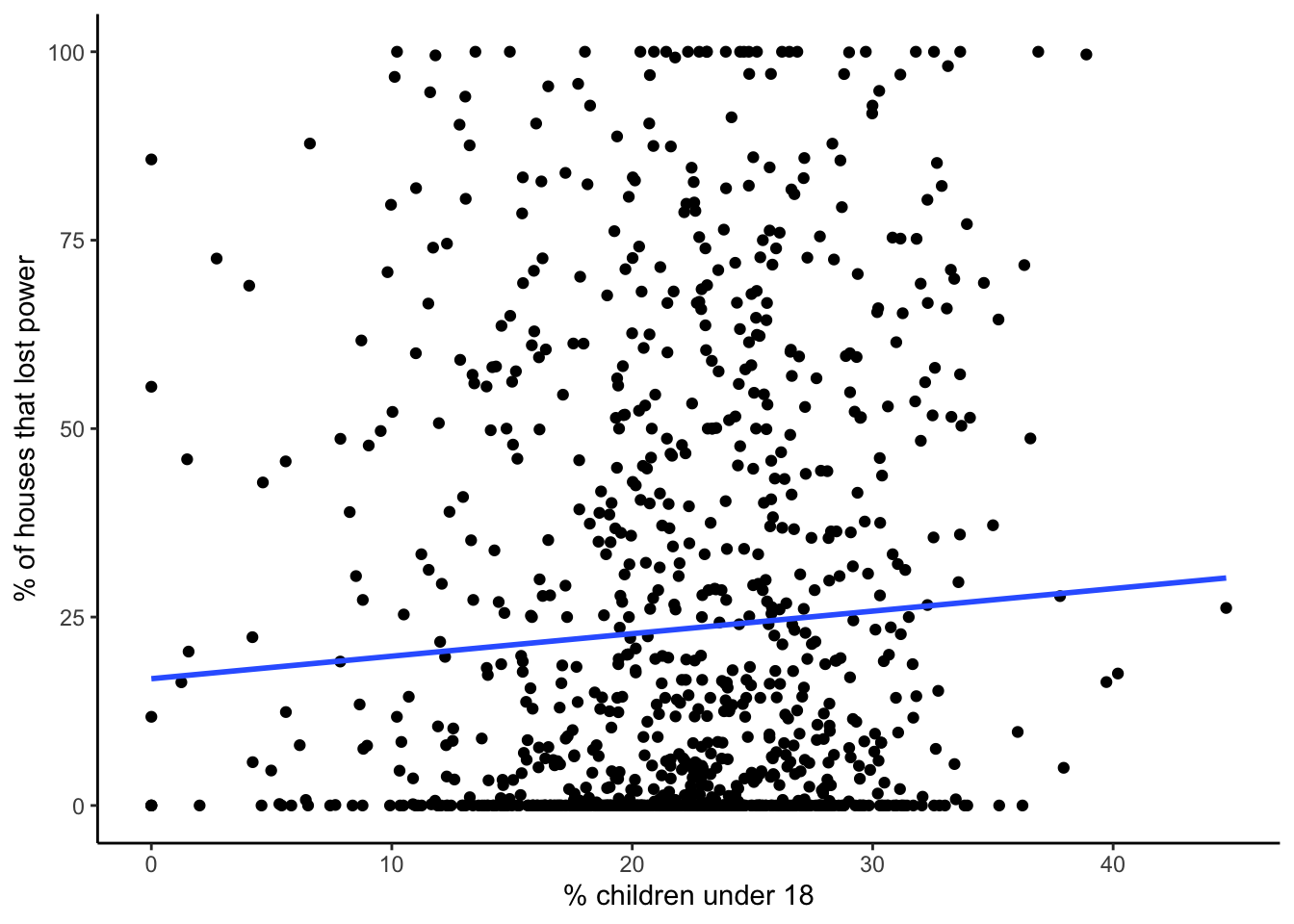
Code for model summary result values
# model summary
summary_model_pct_children_under_18 <- summary(model_pct_children_under_18)

# extract model coefficients
slope_coef_children_under_18 <- round(summary_model_pct_children_under_18$coefficients["pct_children_under_18", "Estimate"], digits = 3)

std_err_children_under_18 <- round(summary_model_pct_children_under_18$coefficients["pct_children_under_18", "Std. Error"], digits = 3)

p_value_children_under_18 <- format(summary_model_pct_children_under_18$coefficients["pct_children_under_18", "Pr(>|t|)"], scientific = FALSE, digits = 2)

# confidence intervals
ci_95_lower_children_under_18 <- round(confint(model_pct_children_under_18, level = 0.95)[2, 1], digits = 3)
ci_95_upper_children_under_18 <- round(confint(model_pct_children_under_18, level = 0.95)[2, 2], digits = 3)

# r-squared value
r_sqrd_children_under_18 <- round(summary_model_pct_children_under_18$r.squared, digits = 3)
Age summary plots
model_plots_age <- (plot_model_pct_65_and_over | plot_model_pct_children_under_18) +
  plot_annotation(title = "Lineral Regression Models of Power Outages vs. Age")

model_plots_age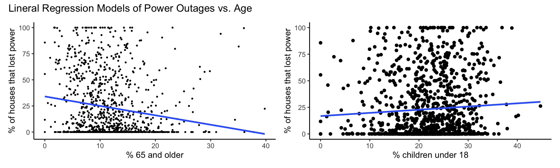
Income
Percent households below poverty
# linear regression model
model_pct_households_below_poverty <- lm(data = blackout_census_data, pct_houses_that_lost_power ~ pct_households_below_poverty)

# plot
plot_model_pct_households_below_poverty <- ggplot(data = blackout_census_data, aes(x = pct_households_below_poverty, y = pct_houses_that_lost_power)) +
  geom_point(size = 0.5) +
  geom_smooth(method = lm, formula = y~x, se = FALSE) +
  theme_classic() +
  labs(x = "% households below poverty", y = "% of houses that lost power")
plot_model_pct_households_below_poverty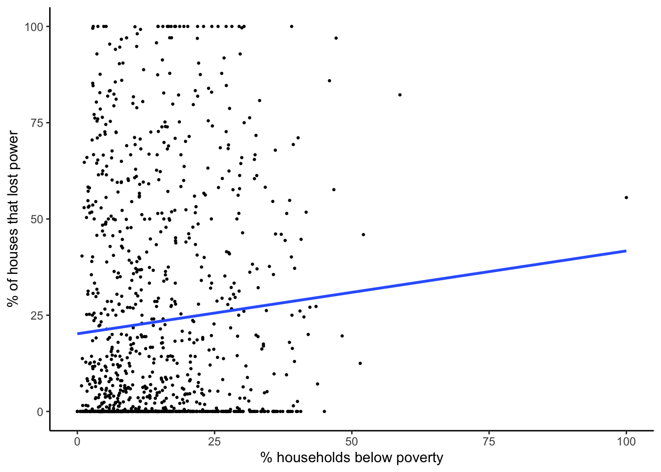
Code for model summary result values
# model summary
summary_model_pct_households_below_poverty <- summary(model_pct_households_below_poverty)

# extract model coefficients
slope_coef_households_below_poverty <- round(summary_model_pct_households_below_poverty$coefficients["pct_households_below_poverty", "Estimate"], digits = 3)

std_err_households_below_poverty <- round(summary_model_pct_households_below_poverty$coefficients["pct_households_below_poverty", "Std. Error"], digits = 3)

p_value_households_below_poverty <- format(summary_model_pct_households_below_poverty$coefficients["pct_households_below_poverty", "Pr(>|t|)"], scientific = FALSE, digits = 2)

# confidence intervals
ci_95_lower_households_below_poverty <- round(confint(model_pct_households_below_poverty, level = 0.95)[2, 1], digits = 3)
ci_95_upper_households_below_poverty <- round(confint(model_pct_households_below_poverty, level = 0.95)[2, 2], digits = 3)

# r-squared value
r_sqrd_households_below_poverty <- round(summary_model_pct_households_below_poverty$r.squared, digits = 3)
Median income
# linear regression model
model_median_income <- lm(data = blackout_census_data, pct_houses_that_lost_power ~ median_income)

# plot
plot_model_median_income <- ggplot(data = blackout_census_data, aes(x = median_income, y = pct_houses_that_lost_power)) +
  geom_point(size = 0.5) +
  geom_smooth(method = lm, formula = y~x, se = FALSE) +
  theme_classic() +
  labs(x = "median income", y = "% of houses that lost power")
plot_model_median_income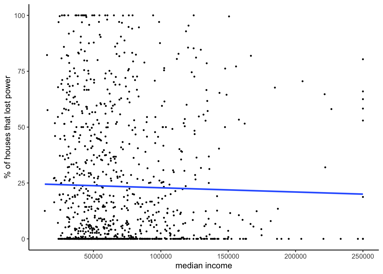
Code for model summary result values
# model summary
summary_model_median_income <- summary(model_median_income)

# extract model coefficients
slope_coef_median_income <- round(summary_model_median_income$coefficients["median_income", "Estimate"], digits = 3)

std_err_median_income <- round(summary_model_median_income$coefficients["median_income", "Std. Error"], digits = 3)

p_value_median_income <- format(summary_model_median_income$coefficients["median_income", "Pr(>|t|)"], scientific = FALSE, digits = 2)

# confidence intervals
ci_95_lower_median_income <- round(confint(model_median_income, level = 0.95)[2, 1], digits = 3)
ci_95_upper_median_income <- round(confint(model_median_income, level = 0.95)[2, 2], digits = 3)

# r-squared value
r_sqrd_median_income <- round(summary_model_median_income$r.squared, digits = 3)
Income summary plots
model_plots_income <- (plot_model_pct_households_below_poverty | plot_model_median_income) +
  plot_annotation(title = "Lineral Regression Models of Power Outages vs. Income")

model_plots_income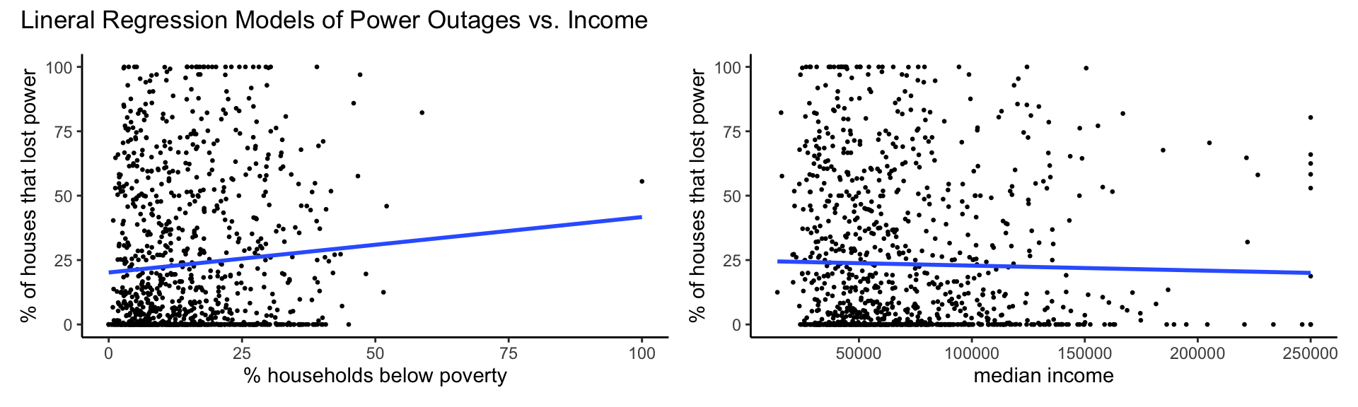
Results
Based on the results of the linear regression models, there is a statistically significant relationship at the 5 % level between percent of houses that lost power and the following variables:
- percent of population white
- percent of population black
- percent of population hispanic / latino
- percent of population age 65 and older
- percent of population children under age 18
- percent of households below the poverty level
Of the significant variables, black; hispanic / latino; children under 18; and poverty were positively correlated with residential power outages. Significant variables that were negatively correlated with residential power outages included white and age 65 and older.
For each model with statistically significant results (ie. p-value < 0.05) we reject the null hypothesis that the socioeconomic variable had no influence on percentage of houses without electricity in each census tract at the 5% level. In other words, the slope coefficient is significantly different from zero. Each slope coefficient represents the change in percent of houses that lost power for a one unit increase in the socioeconomic variable. To use the percent white model as an example, for each one unit increase in percent of census population that is white, the percent of census level residential power outages decreases by 0.168. For the percent white model, the 95% confidence interval for the slope coefficient ranges from -0.251 to -0.085. This means that there is a 95% change that this interval includes the true census level rate of change for percent residential power outages for each one unit change in percent of population that is white.
The r-squared terms represent the variance in percent of houses without power that can be explained by the socioeconomic variable. The r-squared values ranged from 0% for the asian model to 2.9% for the age 65 and older model.
The results of the linear models are summarized in the table below.
Code to create summary table
model_summary_df <- data.frame(model_name = c("white", "black", "native american", "asian", "hispanic / latino", "65 and older", "children under 18", "poverty", "median income"),
                               slope_coef = c(slope_coef_white, slope_coef_black, slope_coef_am_native, slope_coef_asian, slope_coef_hispanic_latino, slope_coef_pct_65_and_over, slope_coef_children_under_18, slope_coef_households_below_poverty, slope_coef_median_income),
                               std_err = c(std_err_white, std_err_black, std_err_am_native, std_err_asian, std_err_hispanic_latino, std_err_pct_65_and_over, std_err_children_under_18, std_err_households_below_poverty, std_err_median_income),
                               p_value = c(p_value_white, p_value_black, p_value_am_native, p_value_asian, p_value_hispanic_latino, p_value_pct_65_and_over, p_value_children_under_18, p_value_households_below_poverty, p_value_median_income),
                               ci_95_lower = c(paste(ci_95_lower_white, "to", ci_95_upper_white),
                                               paste(ci_95_lower_black, "to", ci_95_upper_black),
                                               paste(ci_95_lower_am_native, "to", ci_95_upper_am_native),
                                               paste(ci_95_lower_asian, "to", ci_95_upper_asian),
                                               paste(ci_95_lower_hispanic_latino, "to", ci_95_upper_hispanic_latino),
                                               paste(ci_95_lower_pct_65_and_over, "to", ci_95_upper_pct_65_and_over),
                                               paste(ci_95_lower_children_under_18, "to", ci_95_upper_children_under_18),
                                               paste(ci_95_lower_households_below_poverty, "to", ci_95_upper_households_below_poverty),
                                               paste(ci_95_lower_median_income, "to", ci_95_upper_median_income)),
                               r_squared = c(r_sqrd_white, r_sqrd_black, r_sqrd_am_native, r_sqrd_asian, r_sqrd_hispanic_latino, r_sqrd_65_and_over, r_sqrd_children_under_18, r_sqrd_households_below_poverty, r_sqrd_median_income)) %>%
  mutate(significance = case_when(
    p_value < 0.05 ~ "yes",
    p_value >= 0.05 ~ "no"))

model_summary_table <- model_summary_df %>%
  kable(col.names = c("model name", "slope coefficent", "standard error", "p-value", "95% confidence interval", "r-squared", "significant at 5% level"),
        caption = "Summary of Model Results") %>%
  kable_paper()
model_summary_table| model name | slope coefficent | standard error | p-value | 95% confidence interval | r-squared | significant at 5% level |
|---|---|---|---|---|---|---|
| white | -0.168 | 0.042 | 0.000076 | -0.251 to -0.085 | 0.015 | yes |
| black | 0.167 | 0.048 | 0.00054 | 0.072 to 0.261 | 0.011 | yes |
| native american | 1.010 | 1.162 | 0.38 | -1.27 to 3.29 | 0.001 | no |
| asian | 0.057 | 0.104 | 0.58 | -0.147 to 0.261 | 0.000 | no |
| hispanic / latino | 0.104 | 0.037 | 0.0047 | 0.032 to 0.176 | 0.007 | yes |
| 65 and older | -0.902 | 0.159 | 0.000000019 | -1.214 to -0.589 | 0.029 | yes |
| children under 18 | 0.299 | 0.140 | 0.033 | 0.025 to 0.573 | 0.004 | yes |
| poverty | 0.215 | 0.084 | 0.011 | 0.05 to 0.38 | 0.006 | yes |
| median income | 0.000 | 0.000 | 0.42 | 0 to 0 | 0.001 | no |
The figures below provide a visual comparison of each model result. The bold portion of the line represents the 90% confidence interval and the full line represents the 95% confidnece interval for each slope coefficent estimate.
race_model_summary <- plot_summs(model_pct_white, model_pct_black, model_pct_am_native, model_pct_asian, model_pct_hispanic_latino,
           inner_ci_level = 0.9,
           model.names = c("white", "black", "native american", "asian", "hispanic/latino"))
race_model_summary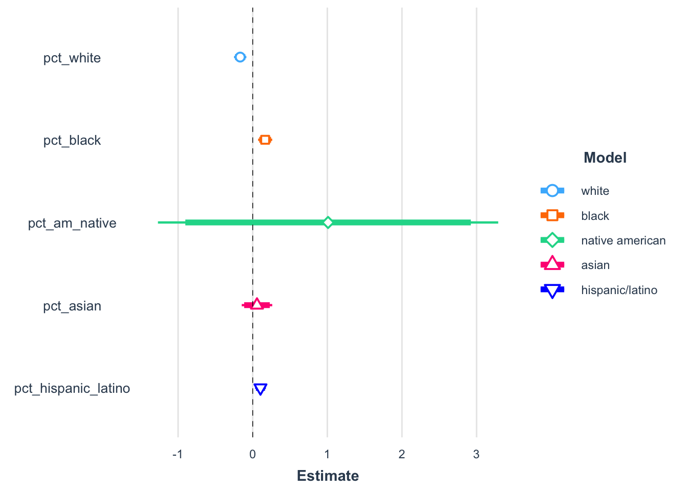
age_model_summary <-plot_summs(model_pct_65_and_over, model_pct_children_under_18,
           inner_ci_level = 0.95,
           model.names = c("over 65", "under 18"))
age_model_summary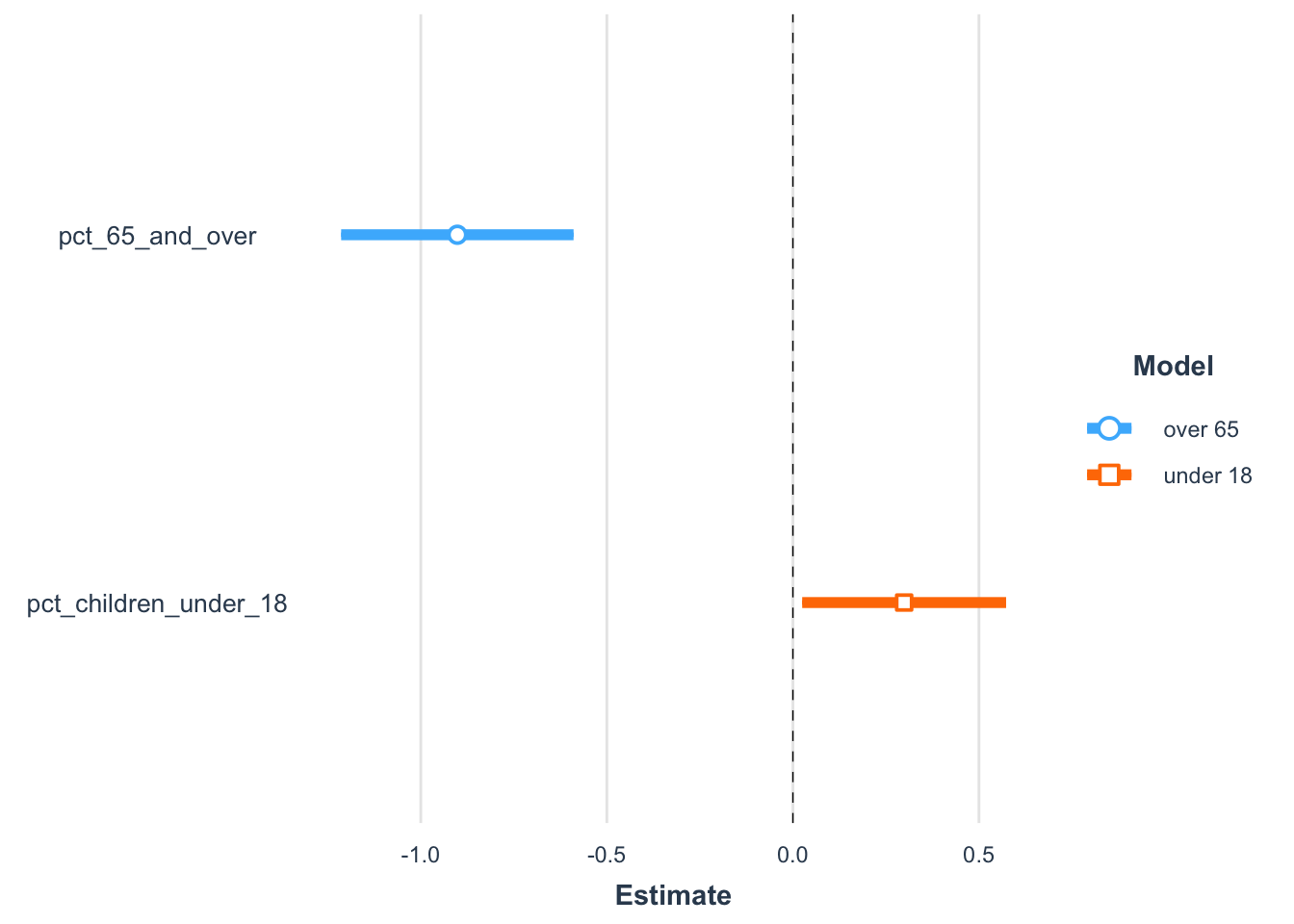
income_model_summary <-plot_summs(model_pct_households_below_poverty, model_median_income,
           inner_ci_level = 0.95,
           model.names = c("poverty", "median income"))
income_model_summary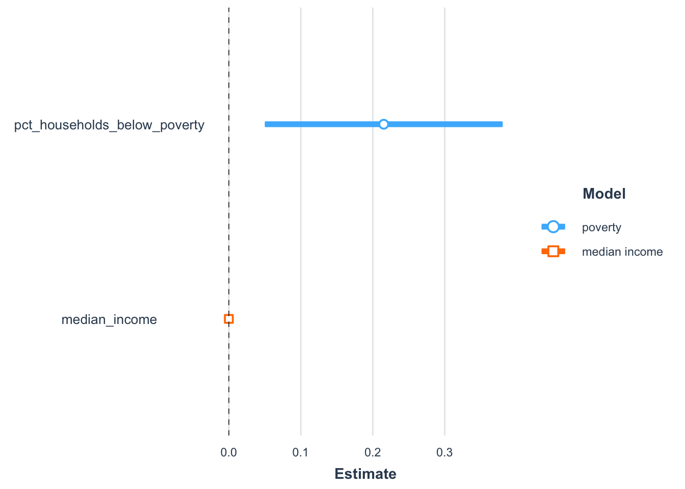
Conclusion
While race, age, and income socioeconomic variables account for only a small portion in the overall variance in residential power outages in the greater Houston area during the February 2021 winter storms, this analysis suggests some racial and economic inequality. Electric utility providers should evaluate power system equipment and infrastructure in areas with higher proportions of people of color and poverty then develop plans to maintain and/or replace critical infrastructure in these areas. The results of this analysis could also be used to provide a more equitable response to future natural disasters.
Note: The purpose of this evaluation was not to predict houses that could be more likely to lose power in the future. This analysis attempts to identify disproportional vulnerabilities of the effected community.