Geospatial Analysis

# load libraries used in analysis
library(tidyverse)
library(here)
library(stars)
library(sf)
library(leaflet)
library(kableExtra)
library(htmlwidgets)
library(htmltools)

Read in satellite imagery

The function below takes an HDFEOS file as input and, from that file, reads the DNB_at_Sensor_Radiance_500m dataset using the stars package. The function then reads the sinusoidal tile x/y positions, adjusts the dimensions, and sets the coordinate reference system.

# function to read and process imagery files as rasters using the stars package
read_dnb_file <- function(file_name) {
  
  # HDF dataset that contains the night lights band
  dataset_name <- "//HDFEOS/GRIDS/VNP_Grid_DNB/Data_Fields/DNB_At_Sensor_Radiance_500m"
  
  # extract the horizontal and vertical tile coordinates from the metadata
  # this information is a string of text
  h_string <- gdal_metadata(file_name)[199]
  v_string <- gdal_metadata(file_name)[219]
  
  # from the horizontal and vertical tile text, obtain the coordinate info as an integer
  tile_h <- as.integer(str_split(h_string, "=", simplify = TRUE)[[2]])
  tile_v <- as.integer(str_split(v_string, "=", simplify = TRUE)[[2]])
  
  # use tile coordinates to calculate a geographic bounding box
  west <- (10 * tile_h) - 180
  north <- 90 - (10 * tile_v)
  east <- west + 10
  south <- north - 10
  
  delta <- 10 / 2400
  
  # read the dataset
  dnb <- read_stars(file_name, sub = dataset_name)
  
  # set the coordinate reference system
  st_crs(dnb) <- st_crs(4326)
  st_dimensions(dnb)$x$delta <- delta
  st_dimensions(dnb)$x$offset <- west
  st_dimensions(dnb)$y$delta <- -delta
  st_dimensions(dnb)$y$offset <- north
  
  return(dnb)
}

# load in files using the read_dnb function
feb7_h08v05_file_name <- "data/VNP46A1/VNP46A1.A2021038.h08v05.001.2021039064328.h5"
dnb_feb7_h08v05 <- read_dnb_file(file_name = feb7_h08v05_file_name)

feb7_h08v06_file_name <- "data/VNP46A1/VNP46A1.A2021038.h08v06.001.2021039064329.h5"
dnb_feb7_h08v06  <- read_dnb_file(file_name = feb7_h08v06_file_name)

feb16_h08v05_file_name <- "data/VNP46A1/VNP46A1.A2021047.h08v05.001.2021048091106.h5"
dnb_feb16_h08v05 <- read_dnb_file(file_name = feb16_h08v05_file_name)

feb16_h08v06_file_name <- "data/VNP46A1/VNP46A1.A2021047.h08v06.001.2021048091105.h5"
dnb_feb16_h08v06 <- read_dnb_file(file_name = feb16_h08v06_file_name)

Combine the tiles from each day using st_mosaic(), like stitching together quit squares.

# combined imagery before the storms
dnb_feb7 <-  st_mosaic(dnb_feb7_h08v05, dnb_feb7_h08v06)

# combined imagery after the storms
dnb_feb16 <- st_mosaic(dnb_feb16_h08v05, dnb_feb16_h08v06)

# extract fill value from metadata
fill_value_string <- gdal_metadata(feb7_h08v05_file_name)[38]
fill_value <- as.integer(str_split(fill_value_string, "=", simplify = TRUE)[[2]])

# convert fill value of 65535 to NA
dnb_feb7[dnb_feb7 == fill_value] = NA
dnb_feb16[dnb_feb16 == fill_value] = NA

Note

At this point you may want to save computer memory by removing objects that wont be used in the rest of the analysis. Unfold the code below to see how to do this.

Code

#remove data not needed anymore
rm(dnb_feb7_h08v05, dnb_feb7_h08v06, dnb_feb16_h08v05, dnb_feb16_h08v06)
gc()

The code below defines and visualizes a bounding box for the region of interest.

# set region on interest
roi <- st_polygon(list(rbind(c(-96.5,29), c(-96.5,30.5), c(-94.5,30.5), c(-94.5,29), c(-96.5,29))))

# set coordinate reference system
roi_sfc <- st_sfc(roi, crs = 4326)
# crs 4326 matches the crs of the satellite imagery

Code for leaflet map

roi_leaflet <- st_as_sf(roi_sfc)
roi_leaflet <- st_make_valid(roi_leaflet)

leaflet(roi_leaflet) %>%
  setView(lat = 29.75, lng = -95.5, zoom = 8) %>%
  addProviderTiles(providers$OpenStreetMap) %>% 
  addPolygons(fillColor = "green", fillOpacity = 0.5, weight = 2)

The next step crops the night light imagery data to the region of interest

dnb_feb7_crop <- st_crop(dnb_feb7, roi_sfc)
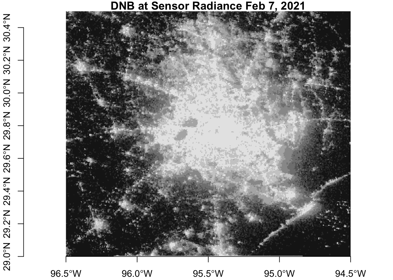
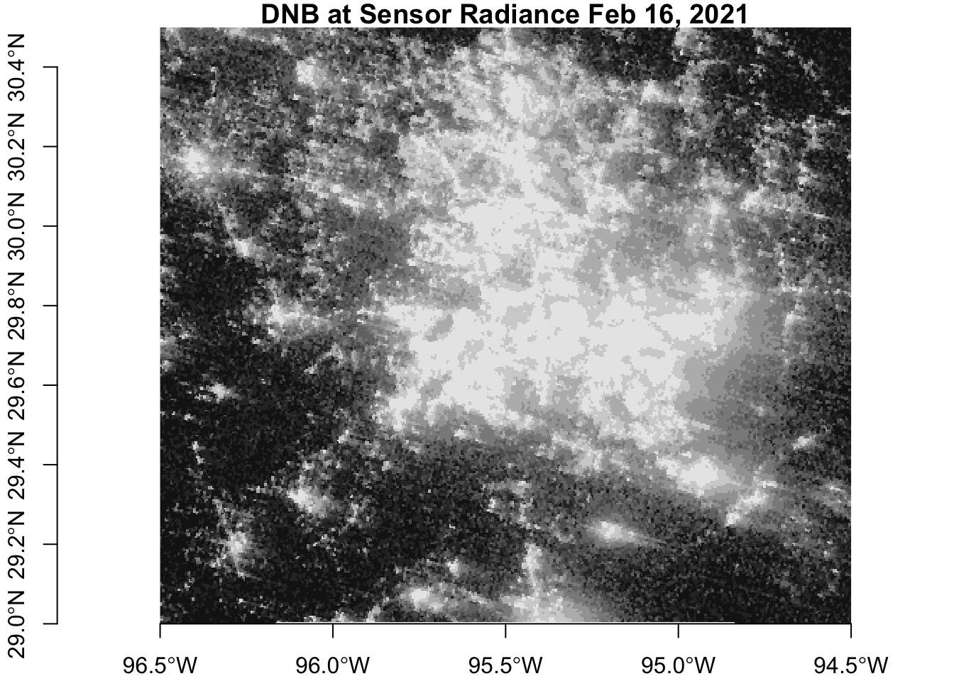
dnb_feb16_crop <- st_crop(dnb_feb16, roi_sfc)

Visualize the data

Before the storms

After the storms

Create blackout mask

A stars raster object representing the difference in night light intensity is created by subtracting the post-storm imagery from the pre-storm imagery. Next, a blackout mask is created to identify areas where night light intensity decreased by more than 200 nW cm-2 sr-1. For this analysis, differences in night light intensity are assumed to be caused by the power outages. The blackout mask is then converted from a stars object to a sf simple features object for use in the rest of the analysis.

night_light_difference <- dnb_feb7 - dnb_feb16

blackout_mask <- night_light_difference
blackout_mask[blackout_mask <= 200] = NA
blackout_mask[blackout_mask > 200] = TRUE

# vectorize the blackout mask
blackout_mask_sf <- st_as_sf(blackout_mask)
blackout_mask_sf_valid <- st_make_valid(blackout_mask_sf)

Next, the blackout mask is cropped to the region of interest and transformed to the NAD83 / Texas Centric Albers Equal Area projection.

blackout_mask_roi <- blackout_mask_sf_valid[roi_sfc, op = st_intersects]

# transform blackout roi to Texas centric albers equal area
blackout_mask_roi_3083 <- st_transform(blackout_mask_roi, crs = 3083)

Road data

Roadway data was obtained from OpenStreetMap. A SQL query and the st_read function were used to load and subset highways and major roads from the full dataset. Since vehicles can be a significant source of observable nighttime light, st_buffer was used to create a 200 meter highway buffer that was then removed from the blackout mask area. This step prevents areas that experienced reduced traffic from being identified as areas with power outages.

# load in roads package and select specifically highways
query_roads <- "SELECT * FROM gis_osm_roads_free_1 WHERE fclass in ('motorway', 'motorway_link', 'primary', 'primary_link')"
highways <- st_read("data/gis_osm_roads_free_1.gpkg", query = query_roads)

# transform to the correct projection
highways_3083 <- st_transform(highways, crs = 3083)

# create a 200 meter buffer
highways_buffer_3083 <- st_buffer(highways_3083, dist = 200) 
highways_buffer_3083 <- st_union(highways_buffer_3083)

# remove the highway buffer from our vectorized blackout mask using st_difference()
blackout_no_highway_3083 <- st_difference(blackout_mask_roi_3083, highways_buffer_3083)

The map below shows the areas identified as still experiencing power outages as of February 16, 2021.

Code for leaflet map

# transform to WG84 to be compatible with the leaflet package
blackout_no_highway_4326 <- st_transform(blackout_no_highway_3083, crs = 4326)

pal_blackout <- colorNumeric(c("red"), 1, na.color = "transparent")

leaflet(blackout_no_highway_4326) %>%
  setView(lat = 29.75, lng = -95.5, zoom = 9) %>%
  addProviderTiles(providers$OpenStreetMap) %>%
  addPolygons(fillColor = ~pal_blackout(DNB_At_Sensor_Radiance_500m), fillOpacity = 0.75, weight = 0)

Note

While the spatial analysis was completed using the NAD83 / Texas Centric Albers Equal Area (EPSG:3083) projection, the processed data was transposed to WGS 84 / World Geodetic System (EPSF:4326) to be compatible with maps created with the leaflet package.

Building data

The building data has previously been cropped to the Houston metroplitan area. A subset of residential buildings is loaded with an SQL query and the st_read function. Close inspection of this data shows many NA values in the type field. When looking at the data on the map, most NA values appear to be residential buildings, but some non-residential buildings such as schools are included.

# read in buildings data and select only residential
query_buildings <- "SELECT *
FROM gis_osm_buildings_a_free_1
WHERE (type IS NULL AND name IS NULL)
OR type in ('residential', 'apartments', 'house', 'static_caravan', 'detached')"

# read buildings gpkg into object, and transform to correct projection
buildings <- st_read("data/gis_osm_buildings_a_free_1.gpkg", query = query_buildings)
buildings_3083 <- st_transform(buildings, crs = 3083)
buildings_4326 <- st_transform(buildings, crs = 4326)

Census data

Socioeconomic data was obtained from the U.S. Census Bureau’s 2019 American Community Survey. This data is aggregated to the census tract level and variables extracted from the full dataset include:

• Race
  • white
  • black
  • native american
  • hispanic / latino
• Age
  • 65 and older
  • children under 18
• Income
  • households below poverty level
  • median income

While the race and age data provides the population of each variable for each census tract, these values were normalized by the total population of the census tract. The poverty data was normalized by number of households in each census tract.

Note

The ACS data consists of the layers listed below, with each layer containing subsets of data as documented in the ACS Metadata.

American Commnity Surey Layer Names

Layer name X01_AGE_AND_SEX X02_RACE X03_HISPANIC_OR_LATINO_ORIGIN X04_ANCESTRY X05_FOREIGN_BORN_CITIZENSHIP X06_PLACE_OF_BIRTH X07_MIGRATION X08_COMMUTING X09_CHILDREN_HOUSEHOLD_RELATIONSHIP X10_GRANDPARENTS_GRANDCHILDREN X11_HOUSEHOLD_FAMILY_SUBFAMILIES X12_MARITAL_STATUS_AND_HISTORY X13_FERTILITY X14_SCHOOL_ENROLLMENT X15_EDUCATIONAL_ATTAINMENT X16_LANGUAGE_SPOKEN_AT_HOME

Layer name X17_POVERTY X18_DISABILITY X19_INCOME X20_EARNINGS X21_VETERAN_STATUS X22_FOOD_STAMPS X23_EMPLOYMENT_STATUS X25_HOUSING_CHARACTERISTICS X27_HEALTH_INSURANCE X28_COMPUTER_AND_INTERNET_USE X29_VOTING_AGE_POPULATION X99_IMPUTATION X24_INDUSTRY_OCCUPATION X26_GROUP_QUARTERS TRACT_METADATA_2019 ACS_2019_5YR_TRACT_48_TEXAS

Census tract geometry

# read in census data geometry
acs_geoms <- st_read("data/ACS_2019_5YR_TRACT_48_TEXAS.gdb",
                     layer = "ACS_2019_5YR_TRACT_48_TEXAS") %>%
  select(-(STATEFP:Shape_Area))

Age and sex layer

# read in variables of interest
acs_age_sex <- st_read("data/ACS_2019_5YR_TRACT_48_TEXAS.gdb",
                      layer = "X01_AGE_AND_SEX")
acs_age_sex_df <- acs_age_sex %>%
  select(GEOID) %>%
  mutate(total_pop_from_age_sex = acs_age_sex$B01001e1,
         median_age = acs_age_sex$B01002e1,
         pop_male_65_66 = acs_age_sex$B01001e20,
         pop_male_67_to_69 = acs_age_sex$B01001e21,
         pop_male_70_to_74 = acs_age_sex$B01001e22,
         pop_male_75_to_79 = acs_age_sex$B01001e23,
         pop_male_80_to_84 = acs_age_sex$B01001e24,
         pop_male_85_and_over = acs_age_sex$B01001e25,
         pop_female_65_66 = acs_age_sex$B01001e44,
         pop_female_67_to_69 = acs_age_sex$B01001e45,
         pop_female_70_to_74 = acs_age_sex$B01001e46,
         pop_female_75_to_79 = acs_age_sex$B01001e47,
         pop_female_80_to_84 = acs_age_sex$B01001e48,
         pop_female_85_and_over = acs_age_sex$B01001e49,
         pop_65_and_over = pop_male_65_66 + pop_male_67_to_69 + pop_male_70_to_74 + pop_male_75_to_79 + pop_male_80_to_84 + pop_male_85_and_over + pop_female_65_66 + pop_female_67_to_69 + pop_female_70_to_74 + pop_female_75_to_79 + pop_female_80_to_84 + pop_female_85_and_over,
         pct_65_and_over = (pop_65_and_over / total_pop_from_age_sex) * 100) %>%
  select(GEOID, total_pop_from_age_sex, pop_65_and_over, pct_65_and_over)

Race layer

acs_race <- st_read("data/ACS_2019_5YR_TRACT_48_TEXAS.gdb",
                      layer = "X02_RACE")
acs_race_df <- acs_race %>%
  select(GEOID) %>%
  mutate(total_pop_from_race = acs_race$B02001e1,
         pop_white = acs_race$B02001e2,
         pct_white = (pop_white / total_pop_from_race) * 100,
         pop_black = acs_race$B02001e3,
         pct_black = (pop_black / total_pop_from_race) * 100,
         pop_am_native = acs_race$B02001e4,
         pct_am_native = (pop_am_native / total_pop_from_race) * 100,
         pop_asian = acs_race$B02001e5,
         pct_asian = (pop_asian / total_pop_from_race) * 100)

Hispanic latino layer

acs_hispanic_latino <- st_read("data/ACS_2019_5YR_TRACT_48_TEXAS.gdb",
                      layer = "X03_HISPANIC_OR_LATINO_ORIGIN")
acs_hispanic_latino_df <- acs_hispanic_latino %>%
  select(GEOID) %>%
  mutate(total_pop_from_hispanic = acs_hispanic_latino$B03002e1,
         pop_hispanic_latino = acs_hispanic_latino$B03002e12,
         pct_hispanic_latino = (pop_hispanic_latino / total_pop_from_hispanic) * 100)

Children and household relationship

acs_children_household <- st_read("data/ACS_2019_5YR_TRACT_48_TEXAS.gdb",
                      layer = "X09_CHILDREN_HOUSEHOLD_RELATIONSHIP")
acs_children_household_df <- acs_children_household %>%
  select(GEOID) %>%
  mutate(pop_children_under_18 = acs_children_household$B09002e1,
         pct_children_under_18 = (pop_children_under_18 / acs_hispanic_latino$B03002e1) * 100)
# the children_household_relationship layer did not contain a total populaiton field

Poverty layer

acs_poverty <- st_read("data/ACS_2019_5YR_TRACT_48_TEXAS.gdb",
                       layer = "X17_POVERTY")
acs_poverty_df <- acs_poverty %>%
  select(GEOID) %>%
  mutate(total_households = acs_poverty$B17017e1,
         num_households_below_poverty = acs_poverty$B17017e2,
         pct_households_below_poverty = (num_households_below_poverty / total_households) * 100)

Income layer

acs_income <- st_read("data/ACS_2019_5YR_TRACT_48_TEXAS.gdb",
                      layer = "X19_INCOME")

acs_income_df <- acs_income %>%
  select(GEOID) %>%
  mutate(median_income = acs_income$B19013e1)

Join census track data

Next, the selected race, age, and income layers are joined. The resulting data set contains the geometry of each census tract and corresponding socioeconomic data.

census_tract_data <- acs_geoms %>%
  left_join(acs_age_sex_df, by = c("GEOID_Data" = "GEOID")) %>%
  left_join(acs_race_df, by = c("GEOID_Data" = "GEOID")) %>%
  left_join(acs_hispanic_latino_df, by = c("GEOID_Data" = "GEOID")) %>%
  left_join(acs_children_household_df, by = c("GEOID_Data" = "GEOID")) %>%
  left_join(acs_poverty_df, by = c("GEOID_Data" = "GEOID")) %>%
  left_join(acs_income_df, by = c("GEOID_Data" = "GEOID")) %>%
  rename(total_population = total_pop_from_age_sex) %>%
  select(-c(total_pop_from_race, total_pop_from_hispanic))

census_tract_data_3083 <- st_transform(census_tract_data, 3083)
census_tract_data_4326 <- st_transform(census_tract_data_3083, crs = 4326)

census_tract_data_roi_4326 <- st_crop(census_tract_data_4326, roi_sfc)
census_tract_data_roi_3083 <- st_transform(census_tract_data_roi_4326, crs = 3083)

Identify houses without power

Houses that lost electricity were identified based on a spatial intersection of the building data and the blackout mask. In this analysis, houses that did not overlap the blackout mask were identified as not losing power (or had power restored by February 16th).

# use spatial subsetting to find all the residential buildings in blackout areas (like we did to crop data to our roi)
blackout_buildings_3083 <- buildings_3083[blackout_no_highway_3083, op = st_intersects]
blackout_buildings_4326 <- st_transform(blackout_buildings_3083, crs = 4326)

# residential houses that did not lose power
no_blackout_buildings_3083 <- setdiff(buildings_3083, blackout_buildings_3083)
no_blackout_buildings_4326 <- st_transform(no_blackout_buildings_3083, crs = 4326)

# use a spatial join to attach the census tract data to the building data
blackout_buildings_census_3083 <- st_join(blackout_buildings_3083, census_tract_data_3083) %>%
  mutate(blackout_status = "lost power")

no_blackout_buildings_census_3083 <- st_join(no_blackout_buildings_3083, census_tract_data_3083) %>%
  mutate(blackout_status = "did not lose power")

number_of_buildings_without_power <- nrow(blackout_buildings_3083)

Based on this analysis, an estimated 144,317 houses in the Houston metropolitan area were without power on February 16, 2021.

all_building_data_3083 <- rbind(blackout_buildings_census_3083, no_blackout_buildings_census_3083)

counts_of_lost_power_by_census_tract <- all_building_data_3083 %>%
  st_drop_geometry() %>%
  group_by(GEOID_Data, blackout_status) %>%
  summarise(count = n()) %>%
  pivot_wider(names_from = blackout_status, values_from = count, values_fill = 0) %>%
  rename(num_houses_did_not_lose_power = "did not lose power",
         num_houses_lost_power = "lost power") %>%
  mutate(pct_houses_that_lost_power = (num_houses_lost_power / (num_houses_did_not_lose_power + num_houses_lost_power)) * 100)

census_tract_blackout_data <- left_join(census_tract_data_roi_4326, counts_of_lost_power_by_census_tract, by = "GEOID_Data")

The map below shows blackout areas layered over census tract populations, with labels identifying the number of houses in each census tract that lost power. The buildings layer was not visualized due to the size of the dataset and slow load times.

Code for leaflet map

pal_pop <- colorQuantile("Blues", census_tract_blackout_data$total_population, n = 5)
pal_blackout <- colorNumeric(c("red"), 1, na.color = "transparent")

pop_colors <- unique(pal_pop(sort(census_tract_blackout_data$total_population)))
pop_labs <- format(quantile(census_tract_blackout_data$total_population, seq(0, 1, .2)), big.mark = ",", digits = 0)
pop_labs <- paste(lag(pop_labs), pop_labs, sep = " - ")[-1]

leaflet(census_tract_blackout_data) %>%
  setView(lat = 29.75, lng = -95.5, zoom = 9) %>%
  addProviderTiles(providers$OpenStreetMap) %>%
  addPolygons(fillColor = ~pal_pop(total_population), fillOpacity = 0.5,
              color = "gray", weight = 0.75,
              label = ~paste("Number of houses without power:", format(num_houses_lost_power, big.mark = ",")),
              highlight = highlightOptions(weight = 2, color = "black", bringToFront = TRUE)) %>%
  addLegend(colors = pop_colors, labels = pop_labs,
            title = "Total Population",
            "bottomright") %>% 
  addPolygons(data = blackout_no_highway_4326, fillColor = ~pal_blackout(DNB_At_Sensor_Radiance_500m), fillOpacity = 0.75, weight = 0)

The final code chunk of this page exports the data that is used for the Statistical Analysis.

# remove spatial info and export to .csv file for use in statistical analysis
census_tract_blackout_data_df <- st_drop_geometry(census_tract_blackout_data) %>% 
  write_csv("data/census_tract_blackout_data_df.csv")