| file name part | explanation |
|---|---|
| VNP46A1 | name of data short product |
| A2021038 | year (ie. 2021) and day of year (ie. 038) that the imagery was acquired |
| h08 | horizontal tile number 8 |
| v05 | vertical tile number 5 |
| 2021039064328 | year (2021), day of year (039), and time (06:43:28 UTC) that the file contents were generated |
| h5 | file extension: HDF-EOS5 (hierarchical data format - earth observing system) |
This analysis evaluates the spatial distribution of power outages in the area surrounding Houston, Texas caused by winter storms in February 2021 and explores which socioeconomic variables are most correlated with power outages. Code and outputs for the geospatial and statistical analyses can be view from the navigation bar at the top of this page.
Note
This analysis started as an assignment for a Spatial Analysis class I took as part of my Masters of Environmental Data Science degree at UC Santa Barbara. Here, the original assignment is expanded upon to include additional socioeconomic variables, a statistical analysis, and interactive leaflet maps.
Background
In 2021, large portions of the United States experience three major winter storms on February 10-11, February 13-17, and February 15-20. The electrical infrastructure in the state of Texas was particularly affected by these events. In the Houston area, an estimated 1.4 million customers were without power on February 15. Using satellite imagery and census data, this analysis quantifies the magnitude and socioeconomic variability of power outages surrounding Houston. Goals of the analysis include:
- estimate the number of homes without power
- evaluate race, age, and income differences between areas with and without power
R libraries
# load libraries used in the R analysis
library(reticulate)
library(tidyverse)
library(kableExtra)
library(here)
library(stars)
library(sf)
library(leaflet)
library(patchwork)
library(jtools)Python packages
# load packages used in Python analysis
import numpy as np
import pandas as pd
import geopandas as gpd
import matplotlib.pyplot as plt
import seaborn as sns
from osgeo import gdal, osr
import rasterio
from rasterio.merge import merge
from rasterio.features import shapes
from shapely.geometry import Polygon
from shapely.geometry import shape
from statsmodels.formula.api import olsGeospatial Analysis
Read in data
Read in all data layers and clip to the region on interest.
Satellite imagery
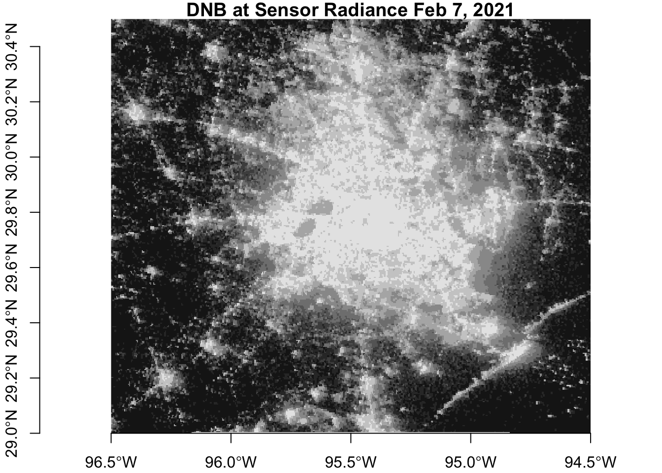
Nighttime light data was obtained from the Visible Infrared Imaging Radiometer Suite (VIIRS), located on the Suomi NPP satellite, which uses a low-light sensor to measure light emissions and reflections. Specifically, the daily at-sensor top of atmosphere (TOA) nighttime radiance (VNP46A1) product was used. This data is available at a 500 meter geographic linear latitude/longitude grid resolution. The processed data accounts for nighttime cloud masks, solar/viewing/lunar geometry values, aerosols, and snow cover. This analysis used the day/night band DNB_At_Sensor_Radiance_500m dataset within the VNP46A1 product.
Imagery from February 7th and February 16th was used to visualize pre- and post-storm conditions due to a lack of cloud cover. Imagery from two tiles was needed to cover the area of interest, which resulted in a total of four files used in the analysis.
- VNP46A1.A2021038.h08v05.001.2021039064328.h5
- VNP46A1.A2021038.h08v06.001.2021039064329.h5
- VNP46A1.A2021047.h08v05.001.2021048091106.h5
- VNP46A1.A2021047.h08v06.001.2021048091105.h5
The functions below takes an HDFEOS file as input and, from that file, reads the DNB_at_Sensor_Radiance_500m dataset. The R code using the stars package with Python code uses GDAL and rasterio. The functions then reads the sinusoidal tile x/y positions, adjusts the dimensions, and sets the coordinate reference system.
Fuctions to read imagery data
# function to read and process imagery files as rasters using the stars package
read_dnb_file <- function(file_name) {
# HDF dataset that contains the night lights band
dataset_name <- "//HDFEOS/GRIDS/VNP_Grid_DNB/Data_Fields/DNB_At_Sensor_Radiance_500m"
# extract the horizontal and vertical tile coordinates from the metadata
# this information is a string of text
h_string <- gdal_metadata(file_name)[199]
v_string <- gdal_metadata(file_name)[219]
# from the horizontal and vertical tile text, obtain the coordinate info as an integer
tile_h <- as.integer(str_split(h_string, "=", simplify = TRUE)[[2]])
tile_v <- as.integer(str_split(v_string, "=", simplify = TRUE)[[2]])
# use tile coordinates to calculate a geographic bounding box
west <- (10 * tile_h) - 180
north <- 90 - (10 * tile_v)
east <- west + 10
south <- north - 10
delta <- 10 / 2400
# read the dataset
dnb <- read_stars(file_name, sub = dataset_name)
# set the coordinate reference system
st_crs(dnb) <- st_crs(4326)
st_dimensions(dnb)$x$delta <- delta
st_dimensions(dnb)$x$offset <- west
st_dimensions(dnb)$y$delta <- -delta
st_dimensions(dnb)$y$offset <- north
return(dnb)
}
# load in files using the read_dnb function
dnb_feb7_h08v05 <- read_dnb_file(file_name = "data/VNP46A1/VNP46A1.A2021038.h08v05.001.2021039064328.h5")
dnb_feb7_h08v06 <- read_dnb_file(file_name = "data/VNP46A1/VNP46A1.A2021038.h08v06.001.2021039064329.h5")
dnb_feb16_h08v05 <- read_dnb_file(file_name = "data/VNP46A1/VNP46A1.A2021047.h08v05.001.2021048091106.h5")
dnb_feb16_h08v06 <- read_dnb_file(file_name = "data/VNP46A1/VNP46A1.A2021047.h08v06.001.2021048091105.h5")# code from: https://blackmarble.gsfc.nasa.gov/tools/OpenHDF5.py
def read_dnb_file_py (file_name):
rasterFiles = file_name
#Get File Name Prefix
rasterFilePre = rasterFiles[8:16] + "_" + rasterFiles[17:23]
rasterPath = "data/VNP46A1/" + rasterFiles
fileExtension = "_BBOX.tif"
# Open HDF file
hdflayer = gdal.Open(rasterPath, gdal.GA_ReadOnly)
# Open raster layer
subhdflayer = hdflayer.GetSubDatasets()[4][0] # DNB_At_Sensor_Radiance_500m
rlayer = gdal.Open(subhdflayer, gdal.GA_ReadOnly)
# Subset the Long Name
outputName = subhdflayer[92:]
outputNameNoSpace = outputName.strip().replace(" ","_").replace("/","_")
outputNameFinal = outputNameNoSpace + "_" + rasterFilePre + fileExtension
# outputFolder = "data/image"
# outputRaster = outputFolder + outputNameFinal
outputFolder = "data/"
outputPre = "image"
outputRaster = outputFolder + outputPre + outputNameFinal
# collect bounding box coordinates
HorizontalTileNumber = int(rlayer.GetMetadata_Dict()["HorizontalTileNumber"])
VerticalTileNumber = int(rlayer.GetMetadata_Dict()["VerticalTileNumber"])
WestBoundCoord = (10*HorizontalTileNumber) - 180
NorthBoundCoord = 90-(10*VerticalTileNumber)
EastBoundCoord = WestBoundCoord + 10
SouthBoundCoord = NorthBoundCoord - 10
# set crs
EPSG = "-a_srs EPSG:4326" #WGS84
translateOptionText = EPSG+" -a_ullr " + str(WestBoundCoord) + " " + str(NorthBoundCoord) + " " + str(EastBoundCoord) + " " + str(SouthBoundCoord)
translateoptions = gdal.TranslateOptions(gdal.ParseCommandLine(translateOptionText))
gdal.Translate(outputRaster, rlayer, options=translateoptions)
return(rasterio.open(outputRaster))
# load in files using the read_dnb function
# this saves geotif files of the data
dnb_feb7_h08v05_py = read_dnb_file_py(file_name = "VNP46A1.A2021038.h08v05.001.2021039064328.h5")
dnb_feb7_h08v06_py = read_dnb_file_py(file_name = "VNP46A1.A2021038.h08v06.001.2021039064329.h5")
dnb_feb16_h08v05_py = read_dnb_file_py(file_name = "VNP46A1.A2021047.h08v05.001.2021048091106.h5")
dnb_feb16_h08v06_py = read_dnb_file_py(file_name = "VNP46A1.A2021047.h08v06.001.2021048091105.h5")Merge imagery files
Combine the tiles from each day, like stitching together quilt squares. The R code uses st_mosaic() and the Python code uses rasterio.merge.
# combined imagery before the storms
feb7_merged <- st_mosaic(dnb_feb7_h08v05, dnb_feb7_h08v06)
# combined imagery after the storms
feb16_merged <- st_mosaic(dnb_feb16_h08v05, dnb_feb16_h08v06)# combined imagery before the storms
feb7_merged_py, transform = merge([dnb_feb7_h08v05_py, dnb_feb7_h08v06_py])
# combined imagery after the storms
feb16_merged_py, transform = merge([dnb_feb16_h08v05_py, dnb_feb16_h08v06_py]) Extract fill value from meta data and convert to NA in data arrays
# extract fill value from metadata
fill_value_string <- gdal_metadata("data/VNP46A1/VNP46A1.A2021038.h08v05.001.2021039064328.h5")[38]
fill_value <- as.integer(str_split(fill_value_string, "=", simplify = TRUE)[[2]])
# convert fill value of 65535 to NA
feb7_merged[feb7_merged == fill_value] = NA
feb16_merged[feb16_merged == fill_value] = NAds = gdal.Open('data/VNP46A1/VNP46A1.A2021038.h08v05.001.2021039064328.h5', gdal.GA_ReadOnly)
meta = ds.GetMetadata()
fill_value_py = int(meta['HDFEOS_GRIDS_VNP_Grid_DNB_Data_Fields_DNB_At_Sensor_Radiance_500m__FillValue'])
# convert fill value to nan
feb7_merged_py = np.where(feb7_merged_py == fill_value_py, np.nan, feb7_merged_py)
feb7_merged_metadata = dnb_feb7_h08v05_py.meta.copy()
feb7_merged_metadata.update(width=feb7_merged_py.shape[2], height=feb7_merged_py.shape[1], transform=transform, dtype='float32')
feb7_merged_dataset = rasterio.io.MemoryFile().open(**feb7_merged_metadata)
feb7_merged_dataset.write(feb7_merged_py)
feb16_merged_py = np.where(feb16_merged_py == fill_value_py, np.nan, feb16_merged_py)
feb16_merged_metadata = dnb_feb16_h08v05_py.meta.copy()
feb16_merged_metadata.update(width=feb16_merged_py.shape[2], height=feb16_merged_py.shape[1], transform=transform, dtype='float64')
feb16_merged_dataset = rasterio.io.MemoryFile().open(**feb16_merged_metadata)
feb16_merged_dataset.write(feb16_merged_py)According to the metadata, the fill value is 65535.
Crop to ROI
# set region on interest
roi_coordinates <- st_polygon(list(rbind(c(-96.5,29), c(-96.5,30.5), c(-94.5,30.5), c(-94.5,29), c(-96.5,29))))
# set coordinate reference system
roi_sfc <- st_sfc(roi_coordinates, crs = 4326)
# crs 4326 matches the crs of the satellite imagery
feb7_roi <- st_crop(feb7_merged, roi_sfc)
feb16_roi <- st_crop(feb16_merged, roi_sfc)roi_coordinates_py = [(-96.5, 29), (-96.5, 30.5), (-94.5, 30.5), (-94.5, 29), (-96.5, 29)]
min_x, min_y = min(coord[0] for coord in roi_coordinates_py), min(coord[1] for coord in roi_coordinates_py)
max_x, max_y = max(coord[0] for coord in roi_coordinates_py), max(coord[1] for coord in roi_coordinates_py)
# Get the window of the ROI
window = feb7_merged_dataset.window(min_x, min_y, max_x, max_y)
# Read the data within the ROI
feb7_roi_py = feb7_merged_dataset.read(window=window)
feb16_roi_py = feb16_merged_dataset.read(window=window)
# Update the transform and profile
transform = feb7_merged_dataset.window_transform(window)
profile = feb7_merged_dataset.profile
profile.update({
'transform': transform,
'width': window.width,
'height': window.height,
'crs': feb7_merged_dataset.crs
})
Code for leaflet map
roi_leaflet <- st_as_sf(roi_sfc)
roi_leaflet <- st_make_valid(roi_leaflet)
leaflet(roi_leaflet) %>%
setView(lat = 29.75, lng = -95.5, zoom = 8) %>%
addProviderTiles(providers$OpenStreetMap) %>%
addPolygons(fillColor = "green", fillOpacity = 0.5, weight = 2)Region of Interest
Before the storms
After the storms

Road and Building data
Building and road data was obtained from OpenStreetMap. Subsets of the data were provided as GeoPackages (.gpkg) for the Houston metropolitan area. SQL queries were used to subset highways and major roads from the the road file and residential buildings from the building file.
Since vehicles can be a significant source of observable nighttime light, a 200 meter highway buffer was removed from the blackout mask area. This step prevents areas that experienced reduced traffic from being identified as areas with power outages.
# load in roads package and select specifically highways
query_roads <- "SELECT * FROM gis_osm_roads_free_1 WHERE fclass in ('motorway', 'motorway_link', 'primary', 'primary_link')"
highways <- st_read("data/gis_osm_roads_free_1.gpkg", query = query_roads)
# transform to the correct projection
highways_3083 <- st_transform(highways, crs = 3083)
# create a 200 meter buffer
highways_buffer_3083 <- st_buffer(highways_3083, dist = 200)
highways_buffer_3083 <- st_union(highways_buffer_3083)
highways_buffer_4326 <- st_transform(highways_buffer_3083, crs = 4326)
highways_buffer_4326 <- st_make_valid(highways_buffer_4326)# load in roads package and select specifically highways
query_roads_py = "SELECT * \
FROM gis_osm_roads_free_1 \
WHERE fclass in ('motorway', 'motorway_link', 'primary', 'primary_link')"
highways_py = gpd.read_file("data/gis_osm_roads_free_1.gpkg", query = query_roads_py)
highways_py = highways_py[(highways_py['fclass'] == 'motorway') | (highways_py['fclass'] == 'motorway_link') | (highways_py['fclass'] == 'primary') | (highways_py['fclass'] == 'primary_link')]
highways_3083_py = highways_py.to_crs(3083)
highway_buffer_3083_py = highways_3083_py.copy()
highway_buffer_3083_py['geometry'] = highway_buffer_3083_py['geometry'].buffer(200)
highway_buffer_3083_py = gpd.GeoDataFrame(geometry=[highway_buffer_3083_py.geometry.unary_union], crs=3083)Close inspection of the building data shows many NA values in the type field. When looking at the data on the map, most NA values appear to be residential buildings, but some non-residential buildings such as schools are included.
# read in buildings data and select only residential
query_buildings <- "SELECT * FROM gis_osm_buildings_a_free_1 WHERE (type IS NULL AND name IS NULL) OR type in ('residential', 'apartments', 'house', 'static_caravan', 'detached')"
# read buildings gpkg into object, and transform to correct projection
buildings <- st_read("data/gis_osm_buildings_a_free_1.gpkg", query = query_buildings)
buildings_3083 <- st_transform(buildings, crs = 3083)
buildings_4326 <- st_transform(buildings, crs = 4326)buildings_4326_py = gpd.read_file('data/gis_osm_buildings_a_free_1.gpkg')
buildings_4326_py = buildings_4326_py[((buildings_4326_py['type'].isna()) & (buildings_4326_py['name'].isna())) | buildings_4326_py['type'].isin(['residential', 'apartments', 'house', 'static_caravan', 'detached'])]
buildings_3083_py = buildings_4326_py.to_crs(3083)del(buildings_4326_py, highways_py, highways_3083_py, query_roads_py)Census data
Data pertaining to race, age, and income demographics for Texas census tract was obtained from the U.S. Census Bureau’s American Community Survey. The data used in this analysis is from 2019 and was cropped to the region of interest. Specific variables evaluated include:
- Race
- white
- black
- native american
- hispanic / latino
- Age
- 65 and older
- children under 18
- Income
- households below poverty level
- median income
While the race and age data provides the population of each variable for each census tract, these values were normalized by the total population of the census tract. The poverty data was normalized by number of households in each census tract.
Note
The ACS data consists of the layers listed below, with each layer containing subsets of data as documented in the ACS Metadata.
|
|
Census tract geometry
# read in census tract geometry
acs_geoms <- st_read("data/ACS_2019_5YR_TRACT_48_TEXAS.gdb",
layer = "ACS_2019_5YR_TRACT_48_TEXAS") %>%
select(-(STATEFP:Shape_Area))# census tract geometry
acs_geoms_py = gpd.read_file('data/ACS_2019_5YR_TRACT_48_TEXAS.gdb',
layer = "ACS_2019_5YR_TRACT_48_TEXAS")
acs_geoms_py_3083 = acs_geoms_py.to_crs(3083)Age and sex layer
# read in variables of interest
acs_age_sex <- st_read("data/ACS_2019_5YR_TRACT_48_TEXAS.gdb",
layer = "X01_AGE_AND_SEX")
acs_age_sex_df <- acs_age_sex %>%
select(GEOID) %>%
mutate(total_pop_from_age_sex = acs_age_sex$B01001e1,
median_age = acs_age_sex$B01002e1,
pop_male_65_66 = acs_age_sex$B01001e20,
pop_male_67_to_69 = acs_age_sex$B01001e21,
pop_male_70_to_74 = acs_age_sex$B01001e22,
pop_male_75_to_79 = acs_age_sex$B01001e23,
pop_male_80_to_84 = acs_age_sex$B01001e24,
pop_male_85_and_over = acs_age_sex$B01001e25,
pop_female_65_66 = acs_age_sex$B01001e44,
pop_female_67_to_69 = acs_age_sex$B01001e45,
pop_female_70_to_74 = acs_age_sex$B01001e46,
pop_female_75_to_79 = acs_age_sex$B01001e47,
pop_female_80_to_84 = acs_age_sex$B01001e48,
pop_female_85_and_over = acs_age_sex$B01001e49,
pop_65_and_over = pop_male_65_66 + pop_male_67_to_69 + pop_male_70_to_74 + pop_male_75_to_79 + pop_male_80_to_84 + pop_male_85_and_over + pop_female_65_66 + pop_female_67_to_69 + pop_female_70_to_74 + pop_female_75_to_79 + pop_female_80_to_84 + pop_female_85_and_over,
pct_65_and_over = (pop_65_and_over / total_pop_from_age_sex) * 100) %>%
select(GEOID, total_pop_from_age_sex, pop_65_and_over, pct_65_and_over)# data for layers of interest
acs_age_sex_py = gpd.read_file('data/ACS_2019_5YR_TRACT_48_TEXAS.gdb',
layer = "X01_AGE_AND_SEX")
acs_age_sex_py = gpd.read_file('data/ACS_2019_5YR_TRACT_48_TEXAS.gdb',
layer = "X01_AGE_AND_SEX")
acs_age_sex_py = acs_age_sex_py.rename(columns={'B01001e1' : 'total_pop_from_age_sex',
'B01002e1' : 'median_age',
'B01001e20' : 'pop_male_65_66',
'B01001e21' : 'pop_male_67_to_69',
'B01001e22' : 'pop_male_70_to_74',
'B01001e23' : 'pop_male_75_to_79',
'B01001e24' : 'pop_male_80_to_84',
'B01001e25' : 'pop_male_85_and_over',
'B01001e44' : 'pop_female_65_66',
'B01001e45' : 'pop_female_67_to_69',
'B01001e46' : 'pop_female_70_to_74',
'B01001e47' : 'pop_female_75_to_79',
'B01001e48' : 'pop_female_80_to_84',
'B01001e49' : 'pop_female_85_and_over'})
acs_age_sex_py['pop_65_and_over'] = acs_age_sex_py['pop_male_65_66'] + acs_age_sex_py['pop_male_67_to_69'] + acs_age_sex_py['pop_male_70_to_74'] + acs_age_sex_py['pop_male_75_to_79'] + acs_age_sex_py['pop_male_80_to_84'] + acs_age_sex_py['pop_male_85_and_over'] + acs_age_sex_py['pop_female_65_66'] + acs_age_sex_py['pop_female_67_to_69'] + acs_age_sex_py['pop_female_70_to_74'] + acs_age_sex_py['pop_female_75_to_79'] + acs_age_sex_py['pop_female_80_to_84'] + acs_age_sex_py['pop_female_85_and_over']
acs_age_sex_py['pct_65_and_over'] = (acs_age_sex_py['pop_65_and_over'] / acs_age_sex_py['total_pop_from_age_sex']) * 100
acs_age_sex_py = acs_age_sex_py[['GEOID', 'total_pop_from_age_sex', 'pop_65_and_over', 'pct_65_and_over']]Race layer
acs_race <- st_read("data/ACS_2019_5YR_TRACT_48_TEXAS.gdb",
layer = "X02_RACE")
acs_race_df <- acs_race %>%
select(GEOID) %>%
mutate(total_pop_from_race = acs_race$B02001e1,
pop_white = acs_race$B02001e2,
pct_white = (pop_white / total_pop_from_race) * 100,
pop_black = acs_race$B02001e3,
pct_black = (pop_black / total_pop_from_race) * 100,
pop_am_native = acs_race$B02001e4,
pct_am_native = (pop_am_native / total_pop_from_race) * 100,
pop_asian = acs_race$B02001e5,
pct_asian = (pop_asian / total_pop_from_race) * 100)acs_race_py = gpd.read_file('data/ACS_2019_5YR_TRACT_48_TEXAS.gdb',
layer = "X02_RACE")
acs_race_py = acs_race_py.rename(columns={'B02001e1' : 'total_pop_from_race',
'B02001e2' : 'pop_white'})
acs_race_py['pct_white'] = (acs_race_py['pop_white'] / acs_race_py['total_pop_from_race']) * 100
acs_race_py['pop_black'] = acs_race_py['B02001e3']
acs_race_py['pct_black'] = (acs_race_py['pop_black'] / acs_race_py['total_pop_from_race']) * 100
acs_race_py['pop_am_native'] = acs_race_py['B02001e4']
acs_race_py['pct_am_native'] = (acs_race_py['pop_am_native'] / acs_race_py['total_pop_from_race']) * 100
acs_race_py['pop_asian'] = acs_race_py['B02001e5']
acs_race_py['pct_asian'] = (acs_race_py['pop_asian'] / acs_race_py['total_pop_from_race']) * 100
acs_race_py = acs_race_py[['GEOID', 'total_pop_from_race', 'pop_white', 'pct_white', 'pop_black', 'pct_black', 'pop_am_native', 'pct_am_native', 'pop_asian', 'pct_asian']]Hispanic latino layer
acs_hispanic_latino <- st_read("data/ACS_2019_5YR_TRACT_48_TEXAS.gdb",
layer = "X03_HISPANIC_OR_LATINO_ORIGIN")
acs_hispanic_latino_df <- acs_hispanic_latino %>%
select(GEOID) %>%
mutate(total_pop_from_hispanic = acs_hispanic_latino$B03002e1,
pop_hispanic_latino = acs_hispanic_latino$B03002e12,
pct_hispanic_latino = (pop_hispanic_latino / total_pop_from_hispanic) * 100)acs_hispanic_latino_py = gpd.read_file('data/ACS_2019_5YR_TRACT_48_TEXAS.gdb',
layer = "X03_HISPANIC_OR_LATINO_ORIGIN")
acs_hispanic_latino_py['total_pop_from_hispanic'] = acs_hispanic_latino_py['B03002e1']
acs_hispanic_latino_py['pop_hispanic_latino'] = acs_hispanic_latino_py['B03002e12']
acs_hispanic_latino_py['pct_hispanic_latino'] = (acs_hispanic_latino_py['pop_hispanic_latino'] / acs_hispanic_latino_py['total_pop_from_hispanic']) * 100
acs_hispanic_latino_py = acs_hispanic_latino_py[['GEOID', 'total_pop_from_hispanic', 'pop_hispanic_latino', 'pct_hispanic_latino']]Children and household relationship
acs_children_household <- st_read("data/ACS_2019_5YR_TRACT_48_TEXAS.gdb",
layer = "X09_CHILDREN_HOUSEHOLD_RELATIONSHIP")
acs_children_household_df <- acs_children_household %>%
select(GEOID) %>%
mutate(pop_children_under_18 = acs_children_household$B09002e1,
pct_children_under_18 = (pop_children_under_18 / acs_hispanic_latino$B03002e1) * 100)
# the children_household_relationship layer did not contain a total population fieldacs_children_household_py = gpd.read_file('data/ACS_2019_5YR_TRACT_48_TEXAS.gdb',
layer = "X09_CHILDREN_HOUSEHOLD_RELATIONSHIP")
acs_children_household_py['pop_children_under_18'] = acs_children_household_py['B09002e1']
acs_children_household_py['pct_children_under_18'] = (acs_children_household_py['pop_children_under_18'] / acs_hispanic_latino_py['total_pop_from_hispanic']) * 100
acs_children_household_py = acs_children_household_py[['GEOID', 'pop_children_under_18', 'pct_children_under_18']]
# the children_household_relationship layer did not contain a total populaiton fieldPoverty layer
acs_poverty <- st_read("data/ACS_2019_5YR_TRACT_48_TEXAS.gdb",
layer = "X17_POVERTY")
acs_poverty_df <- acs_poverty %>%
select(GEOID) %>%
mutate(total_households = acs_poverty$B17017e1,
num_households_below_poverty = acs_poverty$B17017e2,
pct_households_below_poverty = (num_households_below_poverty / total_households) * 100)acs_poverty_py = gpd.read_file('data/ACS_2019_5YR_TRACT_48_TEXAS.gdb',
layer = "X17_POVERTY")
acs_poverty_py['total_households'] = acs_poverty_py['B17017e1']
acs_poverty_py['num_households_below_poverty'] = acs_poverty_py['B17017e2']
acs_poverty_py['pct_households_below_poverty'] = (acs_poverty_py['num_households_below_poverty'] / acs_poverty_py['total_households']) * 100
acs_poverty_py = acs_poverty_py[['GEOID', 'total_households', 'num_households_below_poverty', 'pct_households_below_poverty']]Income layer
acs_income <- st_read("data/ACS_2019_5YR_TRACT_48_TEXAS.gdb",
layer = "X19_INCOME")
acs_income_df <- acs_income %>%
select(GEOID) %>%
mutate(median_income = acs_income$B19013e1)acs_income_py = gpd.read_file('data/ACS_2019_5YR_TRACT_48_TEXAS.gdb',
layer = "X19_INCOME")
acs_income_py['median_income'] = acs_income_py['B19013e1']
acs_income_py = acs_income_py[['GEOID', 'median_income']]Join census track data
Next, the selected race, age, and income layers are joined. The resulting dataset contains the geometry of each census tract and corresponding socioeconomic data.
census_tract_data <- acs_geoms %>%
left_join(acs_age_sex_df, by = c("GEOID_Data" = "GEOID")) %>%
left_join(acs_race_df, by = c("GEOID_Data" = "GEOID")) %>%
left_join(acs_hispanic_latino_df, by = c("GEOID_Data" = "GEOID")) %>%
left_join(acs_children_household_df, by = c("GEOID_Data" = "GEOID")) %>%
left_join(acs_poverty_df, by = c("GEOID_Data" = "GEOID")) %>%
left_join(acs_income_df, by = c("GEOID_Data" = "GEOID")) %>%
rename(total_population = total_pop_from_age_sex) %>%
select(-c(total_pop_from_race, total_pop_from_hispanic))
census_tract_data_3083 <- st_transform(census_tract_data, 3083)
census_tract_data_4326 <- st_transform(census_tract_data_3083, crs = 4326)
census_tract_data_roi_4326 <- st_crop(census_tract_data_4326, roi_sfc)
census_tract_data_roi_3083 <- st_transform(census_tract_data_roi_4326, crs = 3083)# join data layers to census tract geometry
census_tract_data_py = acs_geoms_py_3083.copy()
census_tract_data_py = census_tract_data_py.merge(acs_age_sex_py, how='left', left_on='GEOID_Data', right_on='GEOID')
census_tract_data_py = census_tract_data_py.merge(acs_race_py, how='left', left_on='GEOID_Data', right_on='GEOID')
census_tract_data_py = census_tract_data_py.drop(columns=['GEOID_x', 'GEOID_y'])
census_tract_data_py = census_tract_data_py.merge(acs_hispanic_latino_py, how='left', left_on='GEOID_Data', right_on='GEOID')
census_tract_data_py = census_tract_data_py.merge(acs_children_household_py, how='left', left_on='GEOID_Data', right_on='GEOID')
census_tract_data_py = census_tract_data_py.drop(columns=['GEOID_x', 'GEOID_y'])
census_tract_data_py = census_tract_data_py.merge(acs_poverty_py, how='left', left_on='GEOID_Data', right_on='GEOID')
census_tract_data_py = census_tract_data_py.merge(acs_income_py, how='left', left_on='GEOID_Data', right_on='GEOID')
census_tract_data_py = census_tract_data_py.drop(columns=['GEOID_x', 'GEOID_y'])del(acs_geoms_py, acs_geoms_py_3083, acs_age_sex_py, acs_race_py, acs_hispanic_latino_py, acs_children_household_py, acs_poverty_py, acs_income_py)Create blackout mask
An array was created to represent the difference in night light intensity by subtracting the post-storm imagery from the pre-storm imagery. Next, a blackout threshold is created to identify areas where night light intensity decreased by more than 200 nW cm-2 sr-1. For this analysis, differences in night light intensity are assumed to be caused by the power outages. Areas where the change in light intensity met the threshold were converted to vector format and the highway buffer area was removed.
difference <- feb7_roi - feb16_roi
threshold <- 200
blackout_threshold <- difference
blackout_threshold[blackout_threshold <= threshold] = NA # not a blackout area
blackout_threshold[blackout_threshold > threshold] = TRUE # a blackout area
# vectorize the blackout mask
blackout_threshold_vector <- st_as_sf(blackout_threshold)
blackout_threshold_vector <- st_make_valid(blackout_threshold_vector) %>%
st_transform(crs = 3083)
# remove the highway buffer from the vectorized blackout mask using st_difference()
blackout_mask_3083 <- st_difference(blackout_threshold_vector, highways_buffer_3083)difference_py = feb7_roi_py - feb16_roi_py
threshold_py = 200
blackout_threshold_py = np.where(difference_py <= threshold_py, 0, 1)
blackout_threshold_dataset = rasterio.io.MemoryFile().open(**profile)
blackout_threshold_dataset.write(blackout_threshold_py)
blackout_threshold_data_py = blackout_threshold_dataset.read(1).astype('int16')
# get shapes as GeoJSON-like objects
shapes_gen = shapes(blackout_threshold_data_py, transform=blackout_threshold_dataset.transform, mask = blackout_threshold_data_py != 0)
# convert shapes to Shapely geometries
geometries = [shape(shape_json) for shape_json, _ in shapes_gen]
# create a GeoDataFrame from Shapely geometries
blackout_threshold_vector_py = gpd.GeoDataFrame(geometry=geometries, crs=blackout_threshold_dataset.crs)
blackout_threshold_vector_3083_py = blackout_threshold_vector_py.to_crs(3083)
blackout_mask_3083_py = gpd.overlay(blackout_threshold_vector_3083_py, highway_buffer_3083_py, how='difference')Visualize
The map below shows the areas identified as still experiencing power outages as of February 16, 2021.
Code for leaflet map
# transform to WG84 to be compatible with the leaflet package
blackout_mask_4326 <- st_transform(blackout_mask_3083, crs = 4326)
pal_blackout <- colorNumeric(c("red"), 1, na.color = "transparent")
leaflet(blackout_mask_4326) %>%
setView(lat = 29.75, lng = -95.5, zoom = 9) %>%
addProviderTiles(providers$OpenStreetMap) %>%
addPolygons(fillColor = ~pal_blackout(DNB_At_Sensor_Radiance_500m), fillOpacity = 0.75, weight = 0)
Note
While the spatial analysis was completed using the NAD83 / Texas Centric Albers Equal Area (EPSG:3083) projection, the processed data was transposed to WGS 84 / World Geodetic System (EPSF:4326) to be compatible with maps created with the leaflet package.
Identify houses without power
Houses that lost electricity were identified based on a spatial intersection of the building data and the blackout mask. In this analysis, houses that did not overlap the blackout mask were identified as not losing power (or had power restored by February 16th).
# use spatial subsetting to find all the residential buildings in blackout areas
blackout_buildings_3083 <- buildings_3083[blackout_mask_3083, op = st_intersects]
number_of_buildings_without_power <- nrow(blackout_buildings_3083)blackout_buildings_3083_py = gpd.sjoin(buildings_3083_py, blackout_mask_3083_py, how='inner', op='intersects')sys:1: FutureWarning: The `op` parameter is deprecated and will be removed in a future release. Please use the `predicate` parameter instead.blackout_buildings_3083_py = blackout_buildings_3083_py.drop_duplicates(subset=['osm_id'])
blackout_buildings_3083_py = blackout_buildings_3083_py.drop(columns=['index_right'])Based on this analysis, an estimated 144,317 houses in the Houston metropolitan area were without power on February 16, 2021.
Aggregate residential building outages to census tract level
# use a spatial join to attach the census tract data to the building data
blackout_buildings_census_3083 <- st_join(blackout_buildings_3083, census_tract_data_3083) %>%
mutate(blackout_status = "lost power")
# residential houses that did not lose power
no_blackout_buildings_3083 <- setdiff(buildings_3083, blackout_buildings_3083)
no_blackout_buildings_census_3083 <- st_join(no_blackout_buildings_3083, census_tract_data_3083) %>%
mutate(blackout_status = "did not lose power")
all_building_data_3083 <- rbind(blackout_buildings_census_3083, no_blackout_buildings_census_3083)
counts_of_lost_power_by_census_tract <- all_building_data_3083 %>%
st_drop_geometry() %>%
group_by(GEOID_Data, blackout_status) %>%
summarise(count = n()) %>%
pivot_wider(names_from = blackout_status, values_from = count, values_fill = 0) %>%
rename(num_houses_did_not_lose_power = "did not lose power",
num_houses_lost_power = "lost power") %>%
mutate(pct_houses_that_lost_power = (num_houses_lost_power / (num_houses_did_not_lose_power + num_houses_lost_power)) * 100)
census_tract_blackout_data_with_geometry <- left_join(census_tract_data_roi_4326, counts_of_lost_power_by_census_tract, by = "GEOID_Data")
census_tract_blackout_data <- census_tract_blackout_data_with_geometry %>%
st_drop_geometry()blackout_buildings_census_3083_py = gpd.sjoin(blackout_buildings_3083_py, census_tract_data_py)
blackout_buildings_census_3083_py['blackout_status'] = 'lost power'
no_blackout_buildings_3083_py = buildings_3083_py[~buildings_3083_py['osm_id'].isin(blackout_buildings_3083_py['osm_id'])]
no_blackout_buildings_census_3083_py = gpd.sjoin(no_blackout_buildings_3083_py, census_tract_data_py)
no_blackout_buildings_census_3083_py['blackout_status'] = 'did not lost power'
all_building_data_3083_py = pd.concat([blackout_buildings_census_3083_py, no_blackout_buildings_census_3083_py], axis=0)
counts_of_lost_power_by_census_tract_py = all_building_data_3083_py.copy()
counts_of_lost_power_by_census_tract_py = counts_of_lost_power_by_census_tract_py[['GEOID_Data', 'blackout_status']]
counts_of_lost_power_by_census_tract_py = pd.pivot_table(counts_of_lost_power_by_census_tract_py, index='GEOID_Data', columns='blackout_status', aggfunc=len, fill_value=0)
counts_of_lost_power_by_census_tract_py.columns = ['num_houses_did_not_lose_power', 'num_houses_lost_power']
counts_of_lost_power_by_census_tract_py.reset_index(inplace=True)
census_tract_blackout_data_py = pd.merge(census_tract_data_py, counts_of_lost_power_by_census_tract_py, how='inner', on='GEOID_Data')
census_tract_blackout_data_py['pct_houses_that_lost_power'] = (census_tract_blackout_data_py['num_houses_lost_power'] / (census_tract_blackout_data_py['num_houses_did_not_lose_power'] + census_tract_blackout_data_py['num_houses_lost_power'])) * 100The map below shows blackout areas layered over census tract populations, with labels identifying the number of houses in each census tract that lost power. The buildings layer was not visualized due to the size of the dataset and slow load times.
Code for leaflet map
pal_pop <- colorQuantile("Blues", census_tract_blackout_data_with_geometry$total_population, n = 5)
pal_blackout <- colorNumeric(c("red"), 1, na.color = "transparent")
pop_colors <- unique(pal_pop(sort(census_tract_blackout_data_with_geometry$total_population)))
pop_labs <- format(quantile(census_tract_blackout_data_with_geometry$total_population, seq(0, 1, .2)), big.mark = ",", digits = 0)
pop_labs <- paste(lag(pop_labs), pop_labs, sep = " - ")[-1]
leaflet(census_tract_blackout_data_with_geometry) %>%
setView(lat = 29.75, lng = -95.5, zoom = 9) %>%
addProviderTiles(providers$OpenStreetMap) %>%
addPolygons(fillColor = ~pal_pop(total_population), fillOpacity = 0.5,
color = "gray", weight = 0.75,
label = ~paste("Number of houses without power:", format(num_houses_lost_power, big.mark = ",")),
highlight = highlightOptions(weight = 2, color = "black", bringToFront = TRUE)) %>%
addLegend(colors = pop_colors, labels = pop_labs,
title = "Total Population",
"bottomright") %>%
addPolygons(data = blackout_mask_4326, fillColor = ~pal_blackout(DNB_At_Sensor_Radiance_500m), fillOpacity = 0.75, weight = 0)